Team:British Columbia/Model1

• Home
• Team
  • Team Members
  • Advisors
  • Where We Live
  • Official Profile
• Project
  • Abstract
  • The Story
  • Objectives
• Achievements
  • Achievements
  • Parts
  • Data
  • Americas Jamboree
• Notebook
  • Notebook
  • Protocols
• Safety
• Modeling
  • Beetle Epidemic
  • Monoterpene Production
  • Synthase Structure
• Human practices
  • Mentorship
  • Synthetic Biology Gone Wild
  • Public Perceptions
• Acknowledgements

MODEL 1: Secretion and Production of Monoterpenes in Yeast

OBJECTIVE: To create a model to assay the production of monoterpenes in our genetically engineered yeast cells given that they contain the metabolic genes IDI1, K6R-hmg2, erg20-2 and a monoterpene synthase.
Model Creator: Gurpal Bisra
Model Advisors: Dr. Eric Lagally, Dr. James Piret, Dr. Steve Withers, Dr. Joanne Fox, Shing Zhan, Alina Chan, Rafael Saer

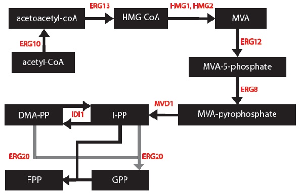
I simplified the mevalonate pathway (Ignea et al. 2011) to only enzymes associated with our project – IDI1, HMG2 and ERG20. I created first order Michaelis-Menten differential equations for the simplified chemical reactions. For this, Dr. Eric Lagally referred me to 2 sources: “Writing Differential Equations” (Bourne 2010) and “Chapter 6- Transport and Kinetics” (Jakubowski 2011). However, many constants and concentrations must be known to solve these differential equations. An enzyme database “BRENDA” contains some kcat and km values (Scheer 2011). However, more research must be done to determine the currently unknown constants. These differential equations can be solved in MATLAB to plot monoterpene concentration as a function of substrate or time.

The Mevalonate Pathway as found in yeast.

Our team wants to mass produce monoterpenes so we...

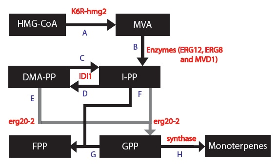
1) Replaced HMG2 with the mutant variant K6R-hmg2, which is stabilized against protein degration (Gardner RG, Hampton RY: A 'distributed degron' allows regulated entry into the ER degradation pathway. Embo J 1999, 18: 5994-6004.)

2) Replaced ERG20 with the mutant variant K197E erg20-2, which produces "25% FPP and 75% GPP instead of 75% FPP and 25% GPP" as compared to the wildtype ERG20 gene (Monoterpenoid biosynthesis in Saccharomyces cerevisiae.). We want more GPP than FPP because our goal is to produce monoterpenes and not diterpenoids (Pathway engineering for functional isoprenoids.).

3) Introduced a gene which encodes for a synthase to use GPP to form monoterpenes. We chose 5 different synthases that each produces different monoterpenes in different proportions (Transcriptome mining, functional characterization, and phylogeny of a large terpene synthase gene family in spruce):

Synthase PgTPS-Pin2 catalyzes GPP into producing 70.5% β-pinene and 29% α-pinene + other monoterpenes in negligible amounts.

Synthase PsTPS-Car1 catalyzes GPP into producing 66.4% 3-carene and 2.7% α-pinene + other monoterpenes in negligible amounts.

Synthase PgxeTPS-Cin catalyzes GPP into producing 65.6% 1,8 cineole, 3.0% α-pinene and 2.6% β-pinene + other monoterpenes in negligible amounts.

Synthase PgTPS-Cin catalyzes GPP into producing 81.1% 1,8 cineole, 1.9% α-pinene and 1.9% β-pinene + other monoterpenes in negligible amounts.

Synthase PsTPS-Pin catalyzes GPP into producing 83.4% α-pinene and 12.6% β-pinene + other monoterpenes in negligible amounts.

Based on these changes, I created a modified model:

Simplified model of the mevalonate pathway with the K6R-hmg2 and erg20-2 genes.

Please note:

1) The enzymes ERG12, ERG8 and MVD1 are NOT RATE LIMITING; therefore, we chose not to include them in our simplified model. However, these enzymes are accounted for in our simulations.

2) The RATE LIMITING STEP is at HMG2.

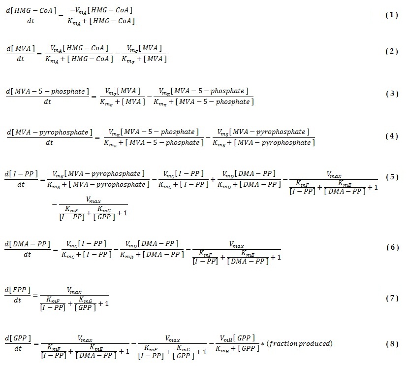
Now, I needed to model these chemical equations as a series of differential equations. As an engineer, I don't have a biochemistry background so this problem was new for me. This website provided the basics to get started. 2 things to take into account are:

1) The direction of the arrow: -if the arrow goes into a component, the equation segment is positive -if the arrow leaves a component, the equation segment is negative

2) Types of Rate Processes -if the rate process is zeroth order, just enter the rate constant -if the rate process i first order, multiply the rate constant by the initial substrate concentration -for a Michaelis-Menten process, include the amount or concentration of the component at the tail of the arrow (call it X1 for example) and you will get: d(X1)/dt = (-Vm*X1)/(Km+X1)

Most of the equations fall under the main 2 types of Michaelis–Menten equations:

The two main types of chemical reactions.

For the first type of reaction, I had to make 2 assumptions:

1) At steady state, [ES] does not change with time, therefore it's derivative with time is = 0. Therefore, k1[E][S] = (k2+k3)[ES]

2) S >> Eo

The second type of Michaelis-Menten kinetic equation applies to cases where I have 2 substrates combining into 1 product via a condensation reaction; DMA-PP and I-PP are condensed to generate geranyl diphosphate (GPP, C10), which is further converted with IPP into ferensyl diphosphate (FPP, C15), with prenyl transferase such as FPP synthase (Pathway engineering for functional isoprenoids.).

To model these types of reactions, I found an expression for the reaction velocity to be: v = d(X)/dt = (Vmax)/( (kms1/[S1]) + (kms2/[S2]) + 1 ) where [S1] = concentration of substrate 1, [S2] = concentration of substrate 2. They have an associated kinetic value. Vmax = kcat*[E] where [E] = the concentration of enzyme.

Differential equations common in all products.

The final thing I needed to consider before writing out the differential equations was how to use data indicating what percentage of monoterpenes were produced. These final steps also took the form of the Michaelis-Menten equations but I modified them by multiplying each by the fraction of product produced. For example, please look at equations 10 and 12 in the differential equations below to see fraction of products are produced for the PgTPS-Pin2 synthase.

The differential equations specific to the PsTPS-Pin synthase, PgTPS-Pin2 synthase, PsTPS-Car1 synthase, PgxeTPS-Cin synthase, PgTPS-Cin synthase.

PARAMETERS - KINETIC CONSTANTS

In order to model each enzyme, at least 2 values must be known: Km and Kcat. These values must be determined when using Michaelis-Menten kinetics to model enzymes.

I found most of my values using the BRENDA database. Not all constants have actually been determined yet for Saccharomyces cerevisiae. After all, our project is based on research that was conducted earlier this year. The values shown in black below were found using the BRENDA database. The values are red had to be inferred. For example, the enzyme HMG2 and K6R-hmg2 were only different in the fact that K6R-hmg2 acted as a stabilizing against protein degration;therefore, the kinetic values for each should be the same. (Gardner RG, Hampton RY: A 'distributed degron' allows regulated entry into the ER degradation pathway. Embo J 1999, 18: 5994-6004.) Also, the values were erg20-2 were determined by deciding that the ratio of kcat/km should be 3 times higher that the same ratio for ERG20. This was based on the fact that erg20-2 has been show to produce "25% FPP and 75% GPP instead of 75% FPP and 25% GPP" as compared to the wildtype ERG20 gene. (Monoterpenoid biosynthesis in Saccharomyces cerevisiae.)

Kcat values for enzymes found in our simplified biochemical pathway.

Km values for enzymes found in our simplified biochemical pathway.

SIMULATIONS

First, I will show you how to simulate the first step of the simplified biochemical pathway using MATLAB. Save the following .m file into MATLAB as named "ex1.m". This program runs under the assumption that time runs from 0 seconds to 100,000 seconds and the initial concentration of substrate = 0 where as the initial concentration of product = 0.

Input the following commands into MATLAB:
>> xspan =[0 100000];
>> ynot = [1 0];
>> [X,Y] = ode45(@ex1,xspan,ynot);
>> plot(X,Y)

OUTPUT:

The concentration of HMG-CoA (blue) and MVA (green) as a function of time.

Now, the above principle can be used to simulate a more complicated pathway. For instance, I could model the simplified version of the biochemical pathway of our engineered yeast cells by coupling all of the differential equations.

Below is a MATLAB code that illustrates how the concentration of β-pinene can be found with one of our engineered yeast cells containing the mutant metabolic genes K6R-hmg2, erg20-2 and the PgTPS-Pin2 synthase gene.

The initial conditions were that time ranged from 0 seconds to 100,000 seconds and the initial concentration of all compounds was 5 moles. The output is a concentration of all compounds found in the biochemical pathway (M) vs. time (s).

To use the code, please save the file as an .m file in MATLAB named "ex2.m" Then, input the following commands into MATLAB while being in the appropriate directory:
>> xspan =[0 100000];
>> ynot = [5 5 5 5 5 5 5 5 5];
>> [X,Y] = ode45(@ex2,xspan,ynot);
>> plot(X,Y)

RESULTS:

The concentration of all compounds found in the biochemical pathway as a function of time.