 "
"
CTRL + E
Signalling is nothing without control...
Contents |
Mathematical modelling: introduction
Mathematical modelling plays nowadays a central role in Synthetic Biology, due to its ability to serve as a crucial link between the concept and realization of a biological circuit: what we propose in this page is a modelling approach to our project, which has proved extremely useful and very helpful before and after the "wet lab".
Thus, immediately at the beginning, when there was little knowledge, a mathematical model based on a system of differential equations was derived and implemented using a set of parameters, so as to validate the feasibility of the project. Once this became clear, starting from the characterization of the single subparts created in the wet lab, some of the parameters of the mathematical model were estimated (the others are known from literature) and they have been fixed to simulate the same model, in order to predict the final behaviour of the whole engineered closed-loop circuit. This approach is consistent with the typical one adopted for the analysis and synthesis of a biological circuit, as exemplified by Pasotti et al 2011.
Therefore here, after a brief overview about the advantages that modelling engineered circuits can bring, we deeply analyze the system of equation formulas, underlining the role and the function of the parameters involved.
Experimental procedures for parameter estimation are discussed and, finally, a different type of circuit is presented. Simulations were performed, using ODEs with MATLAB and used to explain the difference between a closed-loop control system model and an open one.
The importance of mathematical modelling
The purposes of deriving mathematical models for gene networks can be:
Prediction: in the initial steps of the project, a good a-priori identification "in silico" allows to suppose the kinetics of the enzymes (AiiA, Luxi) and HSL involved in our gene network, basically to understand if the complex circuit structure and functioning could be achievable and to investigate the range of parameters values for which the behavior is that expected. (Endler et al, 2009)
Parameter identification: a modellistic approach is helpful to get all the parameters involved, in order to perform realistic simulations not only of the single subparts created, but also of the whole final circuit, according to the a-posteriori identification.
Modularity: studing and characterizing basic BioBrick Parts can allow to reuse this knowledge in other studies, facing with the same basic modules (Braun et al, 2005; Canton et al, 2008).
Equations for gene networks


Hyphotesis of the model
|
HP1: In order to better investigate the range of dynamics of each subparts, every promoter has been
considered with 4 different RBSs, so as to develop more knowledge about the state variables in several configurations
of RBS' efficiency. Hereafter, referring to the notation "RBSx" we mean, respectively,
RBS30,
RBS31,
RBS32,
RBS34.
HP2: In equation (2) only HSL is considered as inducer, instead of the complex LuxR-HSL. This is motivated by the fact that our final device offers a constitutive production of LuxR (due to the upstream constitutive promoter pLac), so that, assuming it abundant in the cytoplasm and always saturated, we can derive the semplification of attributing pLux promoter i nduction only by HSL: this is the reason why we didn' t consider LuxR in the equations system as well as LuxI and AiiA. HP3: in system equation, LuxI and AiiA amounts are expressed per cell. For this reason, the whole equation (3), except for the term of intrinsic degradation of HSL, is multiplied by the number of cells N, due to the property of the lactone to diffuse free inside/outside bacteria. HP4: considering promoters pTet and pLux, we assume their strengths (measured in PoPs), due to a certain concentration of inducer (aTc, HSL for Ptet, Plux respectively) independent from the gene encoding. In other words, in our hypotesis, if we would substitute the mRFP coding region with a region coding for another gene (in our case, AiiA or LuxI), we would obtain the same synthesis rate: this is the reason why the strength of the complex promoter-RBSx is expressed in Arbitrary Units [AUr]. HP5: considering the exponential growth, concentration of the enzymes AiiA and LuxI is supposed to be constant, because the their production in equally compensated by diluition. |
Equations (1) and (2)
Equations (1) and (2) have identical structure, differing only in the parameters involved. They represent the synthesis degradation and diluition of both the enzymes of the circuit, LuxI and AiiA, respectively in the first and second equation: in each of them both transcription and translation processes have been condensed. The corresponding mathematical formalism is analogous to that used by Pasotti et al 2011, Suppl. Inf., even if here we do not model LuxR-HSL complex formation, as explained below.
These equations are composed of 2 parts:
These equations are composed of 2 parts:
- The first term describes, through Hill's equation formalism, the synthesis rate of the protein of interest (either LuxI or AiiA) depending on the concentration of the inducer (anhydrotetracicline -aTc- or HSL respectively), responsable for activating of the regulatory element composed of promoter and RBSx. In the parameter table (see below), α refers to the maximum activation of the promoter, δ stands for its leakage activity (this means that the promoter is quite active even if there is no induction). In particular, in equation (1), the quite total inhibition of pTet promoter is due to the constitutive production of TetR by our MGZ1 strain, while, in equation (2), pLux is almost inactivated in the absence of the complex LuxR-HSL.
Furthermore, in both equations k stands for the dissaciation constant of the promoter from the inducer (respectively aTc and HSL in eq. 1 and 2), while η is the cooperativity constant.
The second term in equations (1) and (2) is in turn composed of 2 parts. The first one (γ*LuxI or γ*AiiA respectively) describes, with an exponential decay, the degradation rate per cell of the protein. The second one (μ*(Nmax-N)/Nmax)*LuxI or μ*(Nmax-N)/Nmax)*AiiA, respectively) takes into account the dilution factor due to cell growth and is related to the cell replication process.
Equation (3)
Here the kinetic of HSL is modeled, basically through enzymatic reactions either related to the production or the degradation of HSL: based on the experiments performed, we derived appropriate expressions for HSL synthesis and degradation. This equation is composed of 3 parts:
- The first term represents the production of HSL due to LuxI expression. We model this process with saturation curve in which Vmax is HSL maximum transcription rate, while kM,LuxI is the dissociation constant of LuxI from the substrate HSL.
- The second term represents the degradation of HSL due to the AiiA expression. Similarly to LuxI, kcat represents maximum degradation per unit of HSL concentration, while kM,AiiA is the concentration at which AiiA dependent HSL concentration rate is (kcat*HSL)/2. The formalism is similar to that found in the Supplementary Information of Danino et al, 2010.
- The third term (γHSL*HSL) is similar to the corresponding ones present in the first two equations and describes the intrinsic protein degradation.
Equation (4)
This is the common logistic cell growth, depending on the rate μ and the maximum number Nmax of cells per well reachable.
Table of parameters and species
| Parameter & Species | Description | Unit of Measurement | Value |
| αpTet | maximum transcription rate of pTet (related with RBSx efficiency) | [(AUr/min)/cell] | - |
| δpTet | leakage factor of promoter pTet basic activity | [-] | - |
| ηpTet | Hill coefficient of pTet | [-] | - |
| kpTet | dissociation costant of aTc from pTet | [nM] | - |
| αpLux | maximum transcription rate of pLux (related with RBSx efficiency) | [(AUr/min)/cell] | - |
| δpLux | leakage factor of promoter pLux basic activity | [-] | - |
| ηpLux | Hill coefficient of pLux | [-] | - |
| kpLux | dissociation costant of HSL from pLux | [nM] | - |
| γpLux | LuxI costant degradation | [1/min] | - |
| γAiiA | AiiA costant degradation | [1/min] | - |
| γHSL | HSL costant degradation | [1/min] | - |
| Vmax | maximum transcription rate of LuxI | [nM/(min*cell)] | - |
| kM,LuxI | dissociation costant of LuxI from HSL | [AUr/cell] | - |
| kcat | maximum number of enzymatic reactions catalysed per minute | [1/(min*cell)] | - |
| kM,AiiA | dissociation costant of AiiA from HSL | [AUr/cell] | - |
| Nmax | maximum number of bacteria per well | [cell] | - |
| μ | rate of bacteria growth | [1/min] | - |
| LuxI | kinetics of enzyme LuxI | [AUr⁄cell] | - |
| AiiA | kinetics of enzyme AiiA | [AUr⁄cell] | - |
| HSL | kinetics of HSL | [nM⁄(min)] | - |
| N | number of cells | cell | - |
Parameter estimation
The philosophy of the model is to predict the behavior of the final closed loop circuit starting from the characterization of single BioBrick parts through a set of well-designed ad hoc experiments. Relating to these, in this section the way parameters of the model have been identified is presented.
As explained before in HP1, considering a set of 4 RBS for each subpart expands the range of dynamics and helps us to understand better the interactions between state variables and parameters.
Promoter (PTet & pLux)

These are the first subparts tested.
In this phase of the project the target is to learn more about promoter pTet and pLux. Characterizing only promoter is quite impossible: for this reason we consider promoter and the respective RBS from RBSx set together (reference to HP1).
As shown in the figure below, we consider a range of induction and we monitor, during the time, absorbance (O.D. stands for "optical density") and fluorescence; the two vertical segments for each graph highlight the exponential phase of bacteria' s growth. Scell (namely, synthesis rate per cell) can be derived as a function of inducer concentration, thereby providing the desired input-output relation (inducer concentration versus promoter+RBS activity), which was modelled as a Hill curve: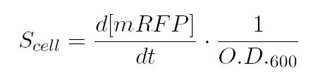 However, also Relative Promoter Unit (RPU) has been calculated as a ratio of Scell of promoter of interest and the Scell of BBa_J23101 (reference to HP4).
 As shown in the figure above, α, as already mentioned, represent the protein maximum synthesis rate, which is reached, in accordance with Hill's formalism, when the inducer concentration tends to infinite, and, more practically, for sufficently high concentrations of inducer, meanwhile the product α*δ stands for the leakage activity (at no induction), liable for protein production (LuxI and AiiA respectively) even in the absence of inducer. The paramenter η is the Hill's cooperativity constant and it affects the rapidity and ripidity of the switch like curve relating Scell with the concentration of inducer.
Lastly, k stands for the semi-saturation constant and, in case of η=1, it indicates the concentration of substrate at which half the synthesis rate is achieved.
As shown in the figure above, α, as already mentioned, represent the protein maximum synthesis rate, which is reached, in accordance with Hill's formalism, when the inducer concentration tends to infinite, and, more practically, for sufficently high concentrations of inducer, meanwhile the product α*δ stands for the leakage activity (at no induction), liable for protein production (LuxI and AiiA respectively) even in the absence of inducer. The paramenter η is the Hill's cooperativity constant and it affects the rapidity and ripidity of the switch like curve relating Scell with the concentration of inducer.
Lastly, k stands for the semi-saturation constant and, in case of η=1, it indicates the concentration of substrate at which half the synthesis rate is achieved.

As shown in the figure below, we consider a range of induction and we monitor, during the time, absorbance (O.D. stands for "optical density") and fluorescence; the two vertical segments for each graph highlight the exponential phase of bacteria' s growth. Scell (namely, synthesis rate per cell) can be derived as a function of inducer concentration, thereby providing the desired input-output relation (inducer concentration versus promoter+RBS activity), which was modelled as a Hill curve:


AiiA & LuxI
In this paragraph is explained how parameters of equation (3) are estimated. The target is to learn the degradation mechanism and production and HSL degradation due to the expression of respectively LuxI and AiiA, in order to estimate Vmax, kM,LuxI, kcat and kM,AiiA parameters. These tests have been performed using the following BioBrick parts:

By now, parameter identification about promoters has already been performed. Furthermore, as explained before, the HP4 is also valid in this case. Moreover, it's possible to quantify exactly the concentration of HSL, using the well-characterized BioBrick BBa_T9002.
 This is a biosensor which receives HSL concentration as input and returns GFP intensity (more precisely Scell) as output. (Canton et al, 2008).
According to this, it' s necessary to get the relationship input-output: so, a "calibration" curve of T9002 is obtain for each test performed.
This is a biosensor which receives HSL concentration as input and returns GFP intensity (more precisely Scell) as output. (Canton et al, 2008).
According to this, it' s necessary to get the relationship input-output: so, a "calibration" curve of T9002 is obtain for each test performed.
So, our idea is to control the degradation of HSL in time. ATc activates pTet and, after, a certain concentration of HSL is introduced. Then, in precise moments, O.D.600 and HSL concentration are monitored using Tecan and T9002 biosensor. Referring to HP5, in exponential growth enzymes equilibrium is conserved.
Due to a well-known induction of aTc, the steady-state level per cell can be calculated:
Referring to HP5, in exponential growth enzymes equilibrium is conserved.
Due to a well-known induction of aTc, the steady-state level per cell can be calculated:
 Then considering, for a determined couple promoter-RBSx, several induction of aTc and, for each of it, several samples of HSL concentration during the time, parameters Vmax, kM,LuxI, kcat and kM,AiiA can be estimated, through numerous iterations of an algorithm implemented in MATLAB.
T. Danino, O. Mondragon-Palomino, L. Tsimring & J. Hasty, "A Synchronized Quorum of Genetic Clocks", Nature vol. 463, pp. 326-330, January 2010.
L. Endler, N. Rodriguez, N. Juty, V. Chelliah, C. Laibe, C. Li and N. Le Novere, "Designing and Encoding Models for Synthetic Biology", Journal of the Royal Society, 2009 Aug 6;6 Suppl 4:S405-17. Epub 2009 Apr 1.
L. Pasotti, M. Quattrocelli, D. Galli, M.G. Cusella De Angelis, P. Magni, "Multiplexing and Demultiplexing Logic Functions for Computing Signal Processing Tasks in Synthetic Biology", Biotechnology Journal, Volume 6,pp. 784-795, 2011.
L. Pasotti, M. Quattrocelli, D. Galli, M.G. Cusella De Angelis, P. Magni, "Multiplexing and Demultiplexing Logic Functions for Computing Signal Processing Tasks in Synthetic Biology, Supporting Information", Biotechnology Journal, Volume 6,available online, 2011.

So, our idea is to control the degradation of HSL in time. ATc activates pTet and, after, a certain concentration of HSL is introduced. Then, in precise moments, O.D.600 and HSL concentration are monitored using Tecan and T9002 biosensor.

N
The parameters Nmax and μ can be calculated from the analysis of the OD600 produced by our MGZ1 culture. In particular, μ is derived as the slope of the log(O.D.600) growth curve. Counting the number of cells of a saturated culture would be quite impossible, so Nmax is determined with a proper procedure. The aim here is to derive the linear proportional coefficient Θ between O.D'.600 and N: this constant can be estimated as the ratio between absorbance (read from TECAN) and the respective number of cells on a petri plate. Finally, Nmax is calcultated as Θ*O.D'.600.
(Pasotti et al, 2010).
Degradation rates
The parameters γLuxI and γAiiA are taken from literature the they contain LVA tag for rapid degradation. Instead, γHSL, approximating HSL kinetics as a decaying exponential, can be derived as the slope of the log(concentration), which can be monitored through BBa_T9002.
Simulations
On a biological level, the ability to control the concentration of a given molecule reveals fundamental in limiting the metabolic burden of the cell; moreover, in the particular case of HSL signalling molecules, this would give the possibility to regulate quorum sensing based population's behaviours. In this section we present some simulations of another circuit, which could validate the concept of cloosed-loop we have discussed so far.
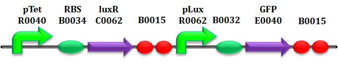
In order to see that, we implemented and simulated in Matlab an open loop circuit, similar to CTRL+E, except for the constitutive production of AiiA.
In order to see that, we implemented and simulated in Matlab an open loop circuit, similar to CTRL+E, except for the constitutive production of AiiA.
 |
 |
References
D. Braun, S. Basu, R. Weiss, "Parameter Estimation for Two Synthetic Gene Networks: a Case Study", ICASSP 2005, vol. 5, v/769 - v/772.
B. Canton, A. Labno and D. Endy, "Refinement and Standardization of Synthetic Biological Parts and Devices", Volume 26, Number 7, July 2008.
B. Canton, A. Labno and D. Endy, "Refinement and Standardization of Synthetic Biological Parts and Devices", Volume 26, Number 7, July 2008.
T. Danino, O. Mondragon-Palomino, L. Tsimring & J. Hasty, "A Synchronized Quorum of Genetic Clocks", Nature vol. 463, pp. 326-330, January 2010.
L. Endler, N. Rodriguez, N. Juty, V. Chelliah, C. Laibe, C. Li and N. Le Novere, "Designing and Encoding Models for Synthetic Biology", Journal of the Royal Society, 2009 Aug 6;6 Suppl 4:S405-17. Epub 2009 Apr 1.
L. Pasotti, M. Quattrocelli, D. Galli, M.G. Cusella De Angelis, P. Magni, "Multiplexing and Demultiplexing Logic Functions for Computing Signal Processing Tasks in Synthetic Biology", Biotechnology Journal, Volume 6,pp. 784-795, 2011.
L. Pasotti, M. Quattrocelli, D. Galli, M.G. Cusella De Angelis, P. Magni, "Multiplexing and Demultiplexing Logic Functions for Computing Signal Processing Tasks in Synthetic Biology, Supporting Information", Biotechnology Journal, Volume 6,available online, 2011.