 "
"
CTRL + E
Signalling is nothing without control...
Contents |
Mathematical modelling page
Mathematical modelling plays nowadays a central role in Synthetic Biology, due to its ability to serve as a crucial link between the concept and realization of a biological circuit: what we propose in this page is a modelling approach to our project, which has proved extremely useful and very helpful before and after the "wet lab".
Thus, immediatly at the beginning, when there was little knowledge, a mathematical model based on a system of differential equations was derived and performed using a set of reasonable parameters, so as to validate the feasibility of the project. Once it became clear, starting from the characterization of the single subparts created in the wet lab, some of the parameters of the mathematical model were estimated (the others are known from literature) and they have been implemented in the same model, in order to predict the final behaviour of the whole engineered closed-loop circuit.
Therefore here, after a brief overview about the advantages that modelling engineered circuits can bring, we deeply analyze the system of equation formulas, underlining the role and the function of the parameters involved.
Experimental procedures for parameters estimation are discussed and, finally, a different type of circuit is presented and simulations performed, using ODE's with MATLAB and explaining the difference between a closed-loop model and an open one.
The importance of the mathematical model
The purposes of writing mathematical models for gene networks can be:
NOTE: In order to investigate better the range of dynamics of each subparts, every promoter has been considered with 4 different RBS, so as to develop more knowledge about the state variables in several configurations of RBS' efficiency. Hereafter, referring to the notation "RBSx" we mean, respectively,
RBS30,
RBS31,
RBS32,
RBS34.
Equations for gene networks


Equations (1) and (2)
Equations (1) and (2) have identical structure, differing only in the parameters involved. They represent the synthesis degradation and diluition of both the enzymes of the circuit, LuxI and AiiA, respectively in the first and second equation: in each of them both transcription and translation processes have been condensed.
These equations are composed of 2 parts:
These equations are composed of 2 parts:
- The first term describes, through Hill's equation formalism, the synthesis rate of the protein of interest (either LuxI or AiiA) depending on the concentration of the inducible protein (anhydrotetracicline -aTc- or HSL respectively). As can be seen in the parameters table (see below),α refers to the maximum activation of the promoter, δ stands for its leakage activity (this means that the promoter is quite active even if there is no induction). In particular, in equation (1), the quite total inhibition of pTet promoter is due to the constitutive production of TetR by our MGZ1 strain, while, in equation (2), pLux is almost repressed in the absence of the complex LuxR-HSL.
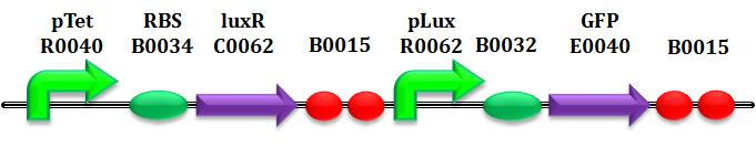
In equation (2) only HSL seems to be the inducer, instead of the complex LuxR-HSL. This is motivated by the fact that our final device offers a constitutive production of LuxR (due to the upstream constitutive promoter pLac), so that, assuming it abundant in the cytoplasm, we can derive the semplification of attributing pLux promoter induction only by HSL: this is the reason why we didn' t consider LuxR in the equations system as well as LuxI and AiiA. Furthermore, in both equations k and η stand respectively for the other parameter of the Hill relationship.
- The second term in equations (1) and (2) is in turn composed of 2 parts. The first one (γ*LuxI or γ*AiiA respectively) describes, with a linear relation, the degradation rate per cell of the protein. The second one (μ*(Nmax-N)/Nmax)*LuxI or μ*(Nmax-N)/Nmax)*AiiA, respectively) takes into account the dilution term due to cell groth phase and is related to the cell replication process.
Equation (3)
Here the kinetics of HSL is modeled, basicly through enzymatic reactions either related to the production or the degradation of HSL: based on the experiments performed, we derived Hill's equation in the case of η=1.
3 parts have been identified in thi equation:
3 parts have been identified in thi equation:
- The first term represents the production of HSL due to the LuxI expression. The parameters involved here are those of a classic Hill equation: Vmax, the maximum transcription rate of the enzyme, and KM, the dissociation constant of....
Moreover, this formula is multiplied by the number of cells N, due to the property of the lactone to diffuse free inside/outside bacteria.
- The second term represents the degradation of HSL due to the AiiA expression. k_cat, KM1....For the same reason of phe first term, this is multiplied too by N.
- The third term (γHSL*HSL) is similar to the corresponding ones present in the first two equations and describes the intrinsic protein degradation.
Equation (4)
This is the common logistic cell growth, depending on the rate μ and the maximum number NMAX of cells per well reachable.
Table of parameters and species
| Parameter & Species | Description | Unit of Measurement | Value |
| αpTet | maximum transcription rate of pTet (related with RBSx efficiency) | [(AUr/min)/cell] | - |
| δpTet | leakage factor of promoter pTet basic activity | [-] | - |
| ηpTet | Hill coefficient of pTet | [-] | - |
| kpTet | dissociation costant of aTc from pTet | [nM] | - |
| αpLux | maximum transcription rate of pLux (related with RBSx efficiency) | [(AUr/min)/cell] | - |
| δpLux | leakage factor of promoter pLux basic activity | [-] | - |
| ηpLux | Hill coefficient of pLux | [-] | - |
| kpLux | dissociation costant of HSL from pLux | [nM] | - |
| γpLux | LuxI costant degradation | [1/min] | - |
| γAiiA | AiiA costant degradation | [1/min] | - |
| γHSL | HSL costant degradation | [1/min] | - |
| Vmax | maximum transcription rate of LuxI | [nM/(min*cell)] | - |
| KM | dissociation costant ? | [AUr/cell] | - |
| Kcat | ?? | [1/(min*cell)] | - |
| KM1 | dissociation costant ? | [AUr/cell] | - |
| Nmax | maximum number of bacteria per well | [cell] | - |
| μ | rate of bacteria growth | [1/min] | - |
| LuxI | kinetics of enzyme LuxI | [AUr⁄cell] | - |
| AiiA | kinetics of enzyme AiiA | [AUr⁄cell] | - |
| HSL | kinetics of HSL | [nM⁄(min)] | - |
| N | number of cells | cell | - |
Parameter estimation
The philosofy of the model is to predict the behavior of the final closed loop circuit starting from the characterization of single BioBrick parts through a set of well-designed ad hoc experiments. Relating to these, in this section the way parameters of the model have been identified is presented.
As explained before in NOTE, considering a set of 4 RBS for each subpart to caracterize increase their range of dynamics and helps us to understand deeplier the interactions between state variables and parameters.
Promoter (PTet & pLux)

These are the first subparts tested.
In this phase of the project the target is to learn more about promoter pTet and pLux. Characterizing only promoter BioBrick is quite impossible: for this reason we consider promoter and the respective RBS from RBSx set together.
Here a strong and reasonable hypothesis must be pointed out: the number of fluorescent protein produced, due to the concentration of induction (aTc, HSL for Ptet, Plux respectively) is exactly the same as the number given by any other protein that would be expressed instead of the mRFP.
In other words, in our hypotesis, if we would substitute the mRFP coding region with a region coding for another protein, we would obtain the same synthesis rate: this is the reason why the strength of the complex promoter-RBSx is expressed in Arbitrary Units [AUr].
As shown in the box below, we consider a range of induction and we monitor, during the time, absorbance (line1, line2) and fluorescence (line3); the two vertical segments for each figure highlight the exponential phase of bacteria' s groth. Scell (explained few lines below) can be derived as a function of inducer concentration, thereby providing the desired input-output relation (inducer concentration versus promoter+RBS activity), which was modelled as a Hill curve.
After that, we can calculate the Scell as: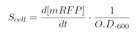 In the end, plotting Scell VS induction, we obtain the activation Hill curve of the considered promoter.
 As shown in the box above, α as already mentioned, represent the protein maximum synthesis rate, which is reached, in accordance with Hill's formalism, when the inducer concentration tends to infinite, and, more practically, for sufficently high concentrations of inducer, meanwhile the product α*δ stands for the leakage activity (at no induction), liable for protein production (LuxI and AiiA respectively) even in the absence of autoinducer. The paramenter η is the Hill's cooperativity constant and it affects the rapidity and ripidity of the switch like curve relating Scell with the concentration of inducer.
Lastly, k stands for the semi-saturation constant and, in case of η=1, it indicates the concentration of substrate at which half the synthesis rate is achieved.
The unities of the various parameters can be easily derived considering the Hill equation(for more details see the Table of parameters above).
As shown in the box above, α as already mentioned, represent the protein maximum synthesis rate, which is reached, in accordance with Hill's formalism, when the inducer concentration tends to infinite, and, more practically, for sufficently high concentrations of inducer, meanwhile the product α*δ stands for the leakage activity (at no induction), liable for protein production (LuxI and AiiA respectively) even in the absence of autoinducer. The paramenter η is the Hill's cooperativity constant and it affects the rapidity and ripidity of the switch like curve relating Scell with the concentration of inducer.
Lastly, k stands for the semi-saturation constant and, in case of η=1, it indicates the concentration of substrate at which half the synthesis rate is achieved.
The unities of the various parameters can be easily derived considering the Hill equation(for more details see the Table of parameters above).

As shown in the box below, we consider a range of induction and we monitor, during the time, absorbance (line1, line2) and fluorescence (line3); the two vertical segments for each figure highlight the exponential phase of bacteria' s groth. Scell (explained few lines below) can be derived as a function of inducer concentration, thereby providing the desired input-output relation (inducer concentration versus promoter+RBS activity), which was modelled as a Hill curve.
After that, we can calculate the Scell as:


AiiA
On a biological level, the ability to control the concentration of a given molecule reveals fundamental in limiting the metabolic burden of the cell; moreover, in the particular case of HSL signalling molecules, this would give the possibility to regulate quorum sensing based population's behaviours.

These experiments aims to learn approximately the degradation rate of HSL due to the expression of AiiA. In this case we are able to quantify exactly the concentration of HSL, using the well-characterized BioBrick BBa_T9002.
 Before discussing parameter estimation, it's good to spend few words abuot this BioBrick. This is a biosensor which receives HSL concentration as input and returns GFP intensity (more precisely SCell) as output.
According to this, it' s necessary to know very well the reationship input-output: a curve of "calibration" of T9002 is obtain for each test performed, even if, in theory, it should be always the same.
So, our idea is to control the degradation of HSL in time reading the fluorescence of T9002 due to a certain concentration of HSL; monitoring it in precise moments since induction (namely, after having waited enough for AiiA to become in stationary phase) and assuming that the concentration follows a decaying exponential, we can estimate the degradation rate.
Kcat represents HSL maximum degradation rate per unit of HSL, reached when AiiA concentration is far above KM1.
KM1 is the dissociation constant between AiiA and HSL.
Before discussing parameter estimation, it's good to spend few words abuot this BioBrick. This is a biosensor which receives HSL concentration as input and returns GFP intensity (more precisely SCell) as output.
According to this, it' s necessary to know very well the reationship input-output: a curve of "calibration" of T9002 is obtain for each test performed, even if, in theory, it should be always the same.
So, our idea is to control the degradation of HSL in time reading the fluorescence of T9002 due to a certain concentration of HSL; monitoring it in precise moments since induction (namely, after having waited enough for AiiA to become in stationary phase) and assuming that the concentration follows a decaying exponential, we can estimate the degradation rate.
Kcat represents HSL maximum degradation rate per unit of HSL, reached when AiiA concentration is far above KM1.
KM1 is the dissociation constant between AiiA and HSL.

The parameters Nmax and μ, can be calculated from the analysis of the OD600 produced by our MGZ1 culture. In particular, μ is derived as the slope of the log(OD600) growth curve. Nmax is determined with a proper procedure. After having reached saturation phase and having retrieved the corresponding OD600, we take a sample of the culture and make serial dilutions of it, then we plate the final diluted culture on a Petri and wait for the formation of colonies. The dilution serves to avoid the growth of too many and too close colonies in the Petri. Finally, we count the number of colonies, which correspond to Nmax.

LuxI
LuxI
The parameters Nmax and μ, can be calculated from the analysis of the OD600 produced by our MGZ1 culture. In particular, μ is derived as the slope of the log(OD600) growth curve. Nmax is determined with a proper procedure. After having reached saturation phase and having retrieved the corresponding OD600, we take a sample of the culture and make serial dilutions of it, then we plate the final diluted culture on a Petri and wait for the formation of colonies. The dilution serves to avoid the growth of too many and too close colonies in the Petri. Finally, we count the number of colonies, which correspond to Nmax.