|
|
| (13 intermediate revisions not shown) |
| Line 5: |
Line 5: |
| | Related Links:</div> | | Related Links:</div> |
| | <div id="boxcontent"><DL> | | <div id="boxcontent"><DL> |
| - | <div class="heading">Vitamin A:</div>
| + | <div class="heading">Modeling:</div><DL> |
| - | <DD><a href="https://2011.igem.org/Team:Johns_Hopkins/Project/VitA">Project</a><br/>
| + | <DD><a href="https://2011.igem.org/Team:Johns_Hopkins/Modeling/Platforms">Modeling Platforms</a><br/> |
| - | <DD><a href="#">Parts</a><br/>
| + | <DD><a href="https://2011.igem.org/Team:Johns_Hopkins/Modeling/LBSMod">LBS Models</a><br/> |
| - | <DD><a href="#">Protocols</a><br/></br/></DL>
| + | <DD><a href="https://2011.igem.org/Team:Johns_Hopkins/Modeling/Opt">Optimization</a><br/> |
| - | <div class="heading">Modeling:</div><DL>
| + | <DD><a href="https://2011.igem.org/Team:Johns_Hopkins/Modeling/Sensitivity">Sensitivity</a><br/> |
| - | <DD><a href="https://2011.igem.org/Team:Johns_Hopkins/Modeling/Platforms">Modeling Platforms</a><br/>
| + | <DD><a href="https://2011.igem.org/Team:Johns_Hopkins/Modeling/ParaFit">Parameter fitting</a><br/></DL> |
| - | <DD><a href="https://2011.igem.org/Team:Johns_Hopkins/Modeling/Methods">Analytic Methods</a><br/>
| + | |
| - | <DD><a href="https://2011.igem.org/Team:Johns_Hopkins/Modeling/GeneExp">Gene Expression</a><br/> | + | |
| - | <DD><a href="https://2011.igem.org/Team:Johns_Hopkins/Modeling/VitA">Vitamin A</a><br/> | + | |
| - | <DD><a href="https://2011.igem.org/Team:Johns_Hopkins/Modeling/VitC">Vitamin C</a><br/></br/></DL> | + | |
| | </div> | | </div> |
| | </div> | | </div> |
| Line 20: |
Line 16: |
| | </html> | | </html> |
| | __NOTOC__ | | __NOTOC__ |
| - | ====== Modeling: Optimization ====== | + | ====== Introduction ====== |
| - | We transition from mathematical description to engineering by using optimization techniques to rationally design the most efficient system that meets our specifications. In our case, we are trying to design a strain of yeast that produces a significant amount of vitamins relative to consensus daily value levels while minimizing the amount of enzyme that the cell needs to produce. Because we are optimizing a very nonlinear objective function in an arbitrary feasible region (parameter space), we investigated a [https://2011.igem.org/Team:Johns_Hopkins/Modeling/OptAlgs series of nonlinear optimization algorithms] with various properties.
| + | Once we sketched out schematic graphical models of vitamin A and vitamin C production, we set out to find the perfect modeling software. We wanted something simple, expressive, powerful, and extendable. We started where [https://2010.igem.org/Team:Edinburgh/Modelling/Kappa last year's modeling prize winner] left off: [http://kappalanguage.org/ Kappa]. |
| - | | + | |
| - | ''In this discussion we consider optimizing the [https://2011.igem.org/Team:Johns_Hopkins/Modeling/VitA β-carotene pathway]. All analysis done for β-carotene has been duplicated for [https://2011.igem.org/Team:Johns_Hopkins/Modeling/VitC l-ascorbate] as well.''
| + | |
| | | | |
| | ====== Objectives ====== | | ====== Objectives ====== |
| - | We have used optimization techniques to answer a number of questions.
| + | * Compare the various modeling languages and platforms available |
| - | * '''What concentration of each enzyme should we attempt to attain in vivo in order to have optimal vitamin production?''' | + | * Use our choice modeling language to develop a generalizable BioBrick model |
| - | * How much vitamin can we expect VitaYeast to produce under different constraints?
| + | |
| - | * What sort of resources will vitamin production demand from the cell?
| + | |
| - | * How will VitaYeast allocate its resources to produce vitamins optimally? | + | |
| - | | + | |
| - | ====== Multi-objective optimization ======
| + | |
| - | ===== Motivation =====
| + | |
| - | We began by hypothesizing what sort of results we could expect from optimizing our pathway for maximum β-carotene production. We quickly realized that we were in for a major problem: from the perspective of the optimization algorithm, adding more enzyme is ''always'' right thing to do. Adding enzyme might increase the pathway's speed and efficiency, but would never cause it to slow down. Thus, any decent algorithm would converge on a solution that pushed the enzyme concentrations to their upper bounds. Running optimization in this way would be trivial.
| + | |
| | | | |
| - | We know intuitively that as we demand increasing enzyme production from cells, we strain their resources until the cell viability and overall product output actually decrease. We do not have a quantitative model for this vague notion of "straining" our VitaYeast, so it cannot be incorporated directly into our simulation. We are left with needing to express the "strain" constraint in a more powerful and dynamic way than bounding and simple linear constraints. One solution is to maximize vitamin production while ''simultaneously'' solving the problem of minimizing "strain". Then, for a given level of strain, we know the optimal vitamin production level and vice-versa.
| + | ====== A BioBrick in Kappa ====== |
| | + | BioBricks are meant to be reusable and composable. While the BioBrick sequences may follow these principles, models of BioBrick-based systems often do not. Ty Thomson's Kappa model is a good example of an attempt to standardize BioBrick model<sup>[[#Foot1|[1]]]</sup>. Thomson's model is designed for use in E. coli, which alone limits its power and would force us to redesign it in our application. However the model suffers from more severe and general drawbacks. In order to take advantage of Kappa's rule-based engine, Thomson creates a general DNA agent with upstream, downstream, and binding sites. Thus any rules applied to DNA will apply to all BioBricks. However, often you want rules to refer to a specific BioBrick. Different BioBricks make different proteins, will be transcribed at different rates, or bind certain repressors. Thomson gets around this problem with a hack: he creates a dummy binding site called "label" and gives it a state such as "BBa000011" to identify the BioBrick. When, for example, a modeler wishes to specify unique transcription rates for each BioBrick, he or she is forced to write the same reaction for each BioBrick, changing only the rate and the state of the label "binding site". While functional, the unattractive nature of this hack points to a fundamental problem in Kappa. |
| | | | |
| - | ===== Pareto Front ===== | + | ====== A BioBrick in LBS ====== |
| | + | Enter LBS's module facility. Modules allow the modeler to ''the structure of a complex interaction once'', and paramaterize that structure with rates, compartments, and agents. Consider the extremely simple gene expression model below adapted from Pedersen's thesis<sup>[[#Foot2|[2]]]. |
| | | | |
| - | Often optimization problems can be phrased as two competing objectives: get home quickly, but use the least gasoline; make the most widgets for the least amount of money. In some cases these problems condense down to a single objective function. For example, widgets can be sold for money, so the single objective function [number of widgets]*[revenue per widget] - [cost of widget production] can be used. When the objective functions cannot be condensed, Pareto frontiers provide a framework to think about the solution to such a problem. Pareto optimality occurs when an improvement in any objective causes a worsening of another objective. Pareto optimality comes from the field of economics, where the optimality condition is phrased as "when making any individual better off requires making someone else worse off". In most problems there exists a surface (the Pareto frontier) in the feasible region which represents the points for which Pareto optimality holds.
| + | <pre> |
| | + | module m(comp nuc; rate trnsc; spec gene, prot){ |
| | + | spec mrna = new{}; |
| | + | nuc[gene + rnap ->{transc} gene + rnap + mrna] | |
| | + | nuc[mrna] ->{1} mrna | |
| | + | rs + mrna ->{0.1} rs +prot |
| | + | }; |
| | + | </pre> |
| | | | |
| - | We are interested in solving the following multi-objective problem: how can we maximize the amount of vitamin produced while minimizing the extra nitrogen required to produce the enzyme. Nitrogen usage serves as a proxy for the general burden of making extra enzymes out of amino acids. We quickly calculated the [https://2011.igem.org/Team:Johns_Hopkins/Modeling/Nitro nitrogen content] of each enzyme in our pathways.
| + | Adding the line m(nucleus, .001, crtI, phytoene_desaturase) will cause gene expression at a specific rate to occur. Unlike in Kappa, this required no "dummy" labeling and no chemical reaction had to be declared. Thus '''the model's abstract structure is totally separated from the realization of that structure for specific systems'''. This module can be reused precisely as it is to model another system. Our BioBrick expression model in LBS makes extensive use of LBS's powerful module facility. |
| | | | |
| - | ===== Execution =====
| + | The following schematic depicts the model we developed in LBS. It was generated in part by [http://lepton.research.microsoft.com/webgec/ Visual GEC], the software environment used to compile and run LBS simulations. |
| - | The first multi-objective optimizer we explored is Matlab's built-in genetic algorithm "gamultiobj", which is based on the NSGA-II algorithm. When we run this optimizer, it generates a population of 100 "individuals" which code for certain enzyme production levels. For each individual a 30-minute simulation of the pathway is run, yielding the β-carotene production level. A separate function figures out how much nitrogen was used. Combined, the β-carotene production and nitrogen usage constitute that population member's "fitness". The algorithm keeps fit individuals and "breeds" them. | + | |
| | | | |
| - | [[Image:Beta-carotene_opto_points.png|thumb|300px|β-carotene pathway Pareto front]] | + | [[File:Expression.jpg|610px|BioBrick expression module implemented in LBS]] |
| | | | |
| - | '''Philosophical side-note:'''<html><br></html>
| + | ===== Expression module ===== |
| - | Consider the fact that we are using a ''genetic'' algorithm to determine which strain of yeast is the most fit with respect to vitamin production. In some sense, we are simulating not just the vitamin production pathway, but the ''entire natural history'' of a synthetic yeast strain, which, until recently, has only existed in silico. Synthetic biology is about bridging the biological-computational gap in both directions: making cells that can compute and making computers that evolve.
| + | We interpret gene expression as a process parameterized by a specific gene and by the specific protein to be made. We also require a compartment to serve as the nucleus, since expression in yeast needs to be compartment-aware. While we take the DNA and protein as given, we declare mRNA in the scope of the expression module. Each gene-protein pair will now get a unique mRNA that is abstracted away from all other interactions in the model. We pass off the work to two sub-modules: transcribe and translate. These modules need not themselves be aware of multiple compartments, so we write a line specifying nuclear export of the mRNA. We also perform RNA degradation in the nucleus in parallel with transcription and in the cytosol in parallel with translation. |
| | + | <pre> |
| | + | module express(comp nuc; spec DNA:{bind}, Prot) { |
| | + | spec mRNA = new{up:binding,down:binding}; |
| | + | nuc[ transcribe(DNA:{bind}, mRNA:{down}) | mRNA ->{rna_deg} ] | |
| | + | nuc[ mRNA ] ->{export} mRNA | |
| | + | translate(mRNA:{up}, Prot) | mRNA -> {rna_deg} |
| | + | }; |
| | + | </pre> |
| | + | ===== Transcription module ===== |
| | + | Transcription requires a DNA segment and an mRNA product. In our model, RNA polymerase, which was declared globally, binds DNA. Then the mRNA molecule appears also bound to RNA polymerase. Finally, the three molecules dissociate. These reactions are irreversible. |
| | + | <pre> |
| | + | module transcribe(spec DNA:{bind}, mRNA:{down}) { |
| | + | RNAP{dna} + DNA{bind} ->{rnap_bind} RNAP{dna!1}-DNA{bind!1} | |
| | + | RNAP{dna!1}-DNA{bind!1} ->{transcription} mRNA{down!2}- |
| | + | RNAP{dna!1,mrna!2}-DNA{bind!1} | |
| | + | mRNA{down!2}-RNAP{dna!1,mrna!2}-DNA{bind!1} ->{termination} |
| | + | mRNA{down} + RNAP{dna,mrna} + |
| | + | DNA{bind} |
| | + | }; |
| | + | </pre> |
| | | | |
| - | After simulating the real-time equivalent of ''years'', the algorithm returns 100 individuals that approximate the Pareto frontier. No individual can make more β-carotene without spending more nitrogen.
| + | ===== Translation module ===== |
| | + | The translation module is similar to and even simpler than transcription. mRNA binds a ribosome (declared globally) in a reversible fashion. Once bound, the ribosome can generate a protein and release both the protein and mRNA in a single step. |
| | + | <pre> |
| | + | module translate(spec mRNA:{up}, Prot) { |
| | + | Ribo{mrna} + mRNA{up} <->{ribo_bind}{ribo_unbind} |
| | + | Ribo{mrna!1}-mRNA{up!1} | |
| | + | Ribo{mrna!1}-mRNA{up!1} ->{translation} Ribo{mrna} + mRNA{up} + Prot |
| | + | }; |
| | + | </pre> |
| | | | |
| - | ====== Allocation analysis ======
| + | Parameters for this model can be found [https://2011.igem.org/Team:Johns_Hopkins/Modeling/Para here]. |
| - | ===== Introduction =====
| + | |
| - | The graphic above tells us a lot about what goes in (nitrogen) and what comes out (β-carotene) of our system, but we are left with somewhat of a black box. We know how much nitrogen gets used and that this usage is optimal, but how does our virtual cell choose to allocate this nitrogen between the various enzymes? What determines this choice? Since the optimizer explicitly minimizes nitrogen usage and maximizes β-carotene production, it seems reasonable that our virtual cell is trying to balance each enzyme's usefulness in synthesizing β-carotene with the nitrogen cost to produce it. Perhaps one of these two factors dominates the decision.
| + | |
| | | | |
| - | [[Image:Bc nitro alloc.png|thumb|300px|β-Carotene nitrogen allocation]]
| + | ====== A Simplified Expression Model ====== |
| | + | The expression model above requires the number of ribosomes and polymerases available to our system, and the various rate constants associated with them, to be estimated. We can measure the final quantity of protein produced and the number of copies of the gene introduced into the cell, but this information is insufficient to estimate all the parameters in the model. Further, literature values regarding these values are sparse, crude, and often contradictory. We decided to build a simplified model with fewer parameters. |
| | | | |
| - | Lets start by looking at how much of each enzyme simulated VitaYeast made as we gave it more nitrogen to work with.
| + | [[File:Simple_expression.jpg|610px|Simplified expression model]] |
| | | | |
| - | As we can see, this plot is pretty noisy. For marginal increases in nitrogen usage, the simulated VitaYeast seems to shift the allocations with a bit of randomness. We interpret this as a result of the model not being very [https://2011.igem.org/Team:Johns_Hopkins/Modeling/Nitro nitrogen content sensitive] to the amounts of enzyme made. Consider adding 1000 nitrogen atoms to the system. That's a difference of only one or two enzyme molecules no matter how it is allocated. The difference between adding it to GGPP_synth_endo versus GGPP_synth_exo is likely erased by rounding error. Thus, for small increases in nitrogen allocation, the simulated VitaYeast is indifferent to how it is allocated, resulting in noise.
| + | This system is so simplistic that it is quite easy to solve for the steady-state concentrations of all species analytically. In fact, we find that if |
| | + | t<sub>s</sub> = transcription rate |
| | + | t<sub>l</sub> = translation rate |
| | + | p = protein degradation rate |
| | + | r = mRNA degradation rate |
| | + | c = number of gene copies in the cell |
| | | | |
| - | [[Image:Bc_nitro_marginal.png|thumb|300px|Marginal nitrogen allocation]] | + | \[[Protein]=(t_{s}\cdot t_{l})/(p\cdot r)\cdot c\] |
| | | | |
| - | ===== Marginal allocation =====
| + | This is useful when translating our pathway optimization results into an implementation strategy for real organisms. We perform our optimization on Matlab models that do not include gene expression. Thus the optimal parameters are stated in terms of enzyme concentrations. Given the target enzyme concentrations suggested by our optimization algorithm, an accurate enough expression model could then allow us to infer optimal gene copy numbers and promoter strengths. We can then search a database of yeast promoter strengths to select the promoter that should be used and the gene copy number needed. In practice this is unrealistic. Predictive models of mRNA lifetime do not exist. Transcription and translation rates are fairly sensitive to the specific codons used. These processes are also exceptionally noisy. It turns out that the metabolic kinetics are much easier to describe accurately, so our results from [https://2011.igem.org/Team:Johns_Hopkins/Modeling/Opt optimization] are useful. However, inferring the genetic construct needed to achieve the optimal protein concentrations will require trial-and-error at the bench. |
| - | Despite the noise, we still see clear overall trends, such as GGPP_synth_endo getting the short end of the stick. We make these trends explicit with a linear fit to each of the curves above. The slope of the fitted curves is the ''marginal nitrogen allocation'', or the portion of each additional unit of nitrogen allocated to each enzyme. A good way to summarize VitaYeast's allocation decisions is to look at the ratios of the marginal allocations below.
| + | |
| | | | |
| - | ===== Normalized marginal allocation ===== | + | ======References====== |
| - | [[Image:Bc nitro marginal frac.png|thumb|300px|Fraction of each nitrogen atom allocated to each enzyme]] | + | <span id="Foot1"><sup>[1]</sup>Ty Thompson. Rule-Based Modeling of BioBrick Parts. http://www.rulebase.org/books/184351-Rule-Based-Modeling-of-BioBrick-Parts.</span> |
| - | The marginal allocation represents the amount of enzyme made, not the actual nitrogen allocation. For example, every molecule of phytoene-cyclase/lycopene-synthase made requires almost twice as much nitrogen as each molecule of endogenous GGPP synthase. To understand exactly where the nitrogen is going, we need to examine the molecule-wise allocation of nitrogen. So we also plot the fraction of a marginal nitrogen atom allocated to each enzyme. We can see that the bifunctional cyclase/synthase receive a very large portion of the nitrogen, both because it is a large enzyme and because it is important, as seen in the marginal allocation above.
| + | |
| | | | |
| - | ===== Conclusions ===== | + | <span id="Foot2"><sup>[2]</sup> Pedersen, M., & Plotkin, G. D. (2010). A language for biochemical systems: Design and formal specification. (C. Priami, R. Breitling, D. Gilbert, M. Heiner, & A. M. Uhrmacher, Eds.)Transactions on Computational Systems Biology XII, 5945, 77-145. Springer Berlin Heidelberg.</span> |
| - | We initially set out to use our optimization results to solve for the genetic construct we would need in order to reproduce optimal VitaYeast in vitro. We have gotten as far as finding the optimal enzyme concentrations needed, but developing an accurate model of enzyme expression from DNA is tricky. VitaYeast uses enzymes not native to yeast. How quickly do these enzymes degrade in their new host? How stable is their mRNA? Without this information, we have little hope of figuring out how to fine-tune our enzyme expression levels. The best we can do is to try to express all the enzymes in the right ratio. Looking at the marginal allocation data, we can see which genes we might be interested in including multiple copies of or using stronger promoters. We believe this rough approximation would be a significant improvement over simply placing all genes in identical constructs. Despite the inability to suggest precise expression parameters, our analysis gave us a good deal of insight into the workings of our pathway. Perhaps this analysis could be applied to natural pathways and larger-scale metabolic networks in order to understand the allocation decisions that drive them.
| + | |
| | | | |
| | | | |
| - | <html> | + | <html></div> |
| - | </div> | + | |
Introduction
Once we sketched out schematic graphical models of vitamin A and vitamin C production, we set out to find the perfect modeling software. We wanted something simple, expressive, powerful, and extendable. We started where last year's modeling prize winner left off: Kappa.
Objectives
- Compare the various modeling languages and platforms available
- Use our choice modeling language to develop a generalizable BioBrick model
A BioBrick in Kappa
BioBricks are meant to be reusable and composable. While the BioBrick sequences may follow these principles, models of BioBrick-based systems often do not. Ty Thomson's Kappa model is a good example of an attempt to standardize BioBrick model[1]. Thomson's model is designed for use in E. coli, which alone limits its power and would force us to redesign it in our application. However the model suffers from more severe and general drawbacks. In order to take advantage of Kappa's rule-based engine, Thomson creates a general DNA agent with upstream, downstream, and binding sites. Thus any rules applied to DNA will apply to all BioBricks. However, often you want rules to refer to a specific BioBrick. Different BioBricks make different proteins, will be transcribed at different rates, or bind certain repressors. Thomson gets around this problem with a hack: he creates a dummy binding site called "label" and gives it a state such as "BBa000011" to identify the BioBrick. When, for example, a modeler wishes to specify unique transcription rates for each BioBrick, he or she is forced to write the same reaction for each BioBrick, changing only the rate and the state of the label "binding site". While functional, the unattractive nature of this hack points to a fundamental problem in Kappa.
A BioBrick in LBS
Enter LBS's module facility. Modules allow the modeler to the structure of a complex interaction once, and paramaterize that structure with rates, compartments, and agents. Consider the extremely simple gene expression model below adapted from Pedersen's thesis[2].
module m(comp nuc; rate trnsc; spec gene, prot){
    spec mrna = new{};
    nuc[gene + rnap ->{transc} gene + rnap + mrna] |
    nuc[mrna] ->{1} mrna |
    rs + mrna ->{0.1} rs +prot
};
Adding the line m(nucleus, .001, crtI, phytoene_desaturase) will cause gene expression at a specific rate to occur. Unlike in Kappa, this required no "dummy" labeling and no chemical reaction had to be declared. Thus the model's abstract structure is totally separated from the realization of that structure for specific systems. This module can be reused precisely as it is to model another system. Our BioBrick expression model in LBS makes extensive use of LBS's powerful module facility.
The following schematic depicts the model we developed in LBS. It was generated in part by Visual GEC, the software environment used to compile and run LBS simulations.
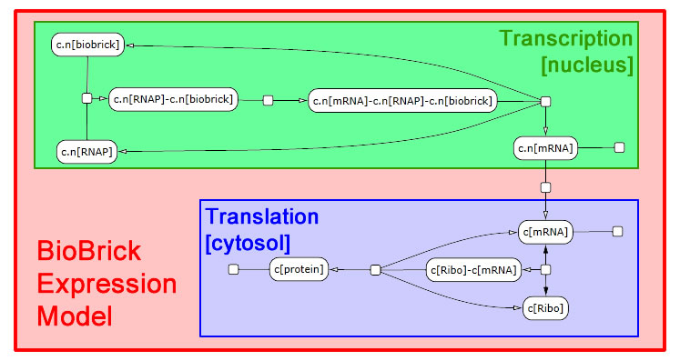
Expression module
We interpret gene expression as a process parameterized by a specific gene and by the specific protein to be made. We also require a compartment to serve as the nucleus, since expression in yeast needs to be compartment-aware. While we take the DNA and protein as given, we declare mRNA in the scope of the expression module. Each gene-protein pair will now get a unique mRNA that is abstracted away from all other interactions in the model. We pass off the work to two sub-modules: transcribe and translate. These modules need not themselves be aware of multiple compartments, so we write a line specifying nuclear export of the mRNA. We also perform RNA degradation in the nucleus in parallel with transcription and in the cytosol in parallel with translation.
module express(comp nuc; spec DNA:{bind}, Prot) {
	spec mRNA = new{up:binding,down:binding};
	nuc[ transcribe(DNA:{bind}, mRNA:{down}) | mRNA ->{rna_deg} ] |
	nuc[ mRNA ] ->{export} mRNA |
	translate(mRNA:{up}, Prot) | mRNA -> {rna_deg}
};
Transcription module
Transcription requires a DNA segment and an mRNA product. In our model, RNA polymerase, which was declared globally, binds DNA. Then the mRNA molecule appears also bound to RNA polymerase. Finally, the three molecules dissociate. These reactions are irreversible.
module transcribe(spec DNA:{bind}, mRNA:{down}) {
	RNAP{dna} + DNA{bind} ->{rnap_bind} RNAP{dna!1}-DNA{bind!1} |
	RNAP{dna!1}-DNA{bind!1} ->{transcription} mRNA{down!2}-
RNAP{dna!1,mrna!2}-DNA{bind!1} |
	mRNA{down!2}-RNAP{dna!1,mrna!2}-DNA{bind!1} ->{termination}
mRNA{down} + RNAP{dna,mrna} +
DNA{bind}
};
Translation module
The translation module is similar to and even simpler than transcription. mRNA binds a ribosome (declared globally) in a reversible fashion. Once bound, the ribosome can generate a protein and release both the protein and mRNA in a single step.
module translate(spec mRNA:{up}, Prot) {
	Ribo{mrna} + mRNA{up} <->{ribo_bind}{ribo_unbind}
Ribo{mrna!1}-mRNA{up!1} |
	Ribo{mrna!1}-mRNA{up!1} ->{translation} Ribo{mrna} + mRNA{up} + Prot
};
Parameters for this model can be found here.
A Simplified Expression Model
The expression model above requires the number of ribosomes and polymerases available to our system, and the various rate constants associated with them, to be estimated. We can measure the final quantity of protein produced and the number of copies of the gene introduced into the cell, but this information is insufficient to estimate all the parameters in the model. Further, literature values regarding these values are sparse, crude, and often contradictory. We decided to build a simplified model with fewer parameters.

This system is so simplistic that it is quite easy to solve for the steady-state concentrations of all species analytically. In fact, we find that if
ts = transcription rate
tl = translation rate
p = protein degradation rate
r = mRNA degradation rate
c = number of gene copies in the cell
\[[Protein]=(t_{s}\cdot t_{l})/(p\cdot r)\cdot c\]
This is useful when translating our pathway optimization results into an implementation strategy for real organisms. We perform our optimization on Matlab models that do not include gene expression. Thus the optimal parameters are stated in terms of enzyme concentrations. Given the target enzyme concentrations suggested by our optimization algorithm, an accurate enough expression model could then allow us to infer optimal gene copy numbers and promoter strengths. We can then search a database of yeast promoter strengths to select the promoter that should be used and the gene copy number needed. In practice this is unrealistic. Predictive models of mRNA lifetime do not exist. Transcription and translation rates are fairly sensitive to the specific codons used. These processes are also exceptionally noisy. It turns out that the metabolic kinetics are much easier to describe accurately, so our results from optimization are useful. However, inferring the genetic construct needed to achieve the optimal protein concentrations will require trial-and-error at the bench.
References
 "
"


