Stochastic Analysis

Insert overview of page here

Method

Insert overview of page here

Simulation

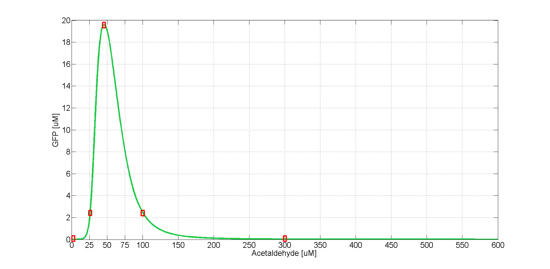
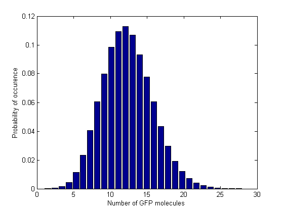
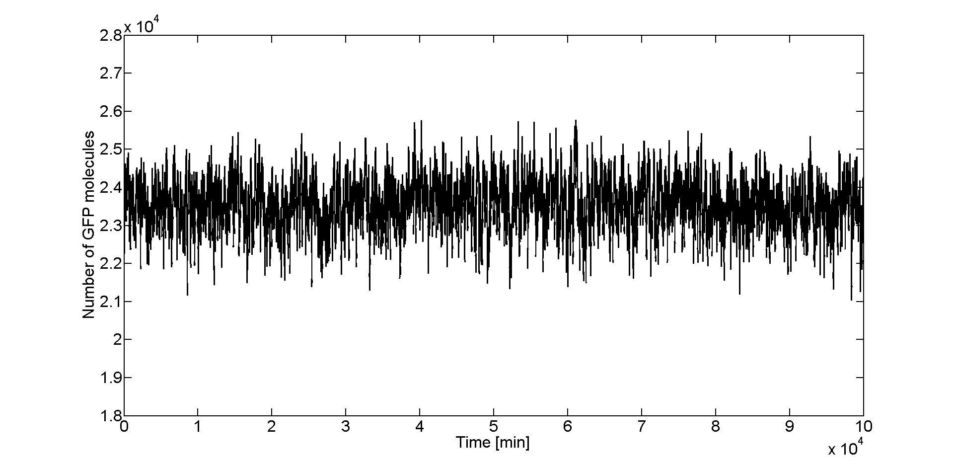
Besides the parameter space search, we performed another type of analysis in order to verify that our system is robust and that it is not bistable. We were especially interested at the GFP band and whether it is always there. We did stochastic simulations to see how our system reacts to noise and how it responds to perturbations. For a certain acetaldehyde concentration (which gives the peak of the band) we wanted to see how the GFP peak value varies over long time period when we consider stochasticity. For the stochastic simulations we used the software Dizzy, to which we gave as an input file an SMBL file with the description of our system. Moving from deteministic to stochastic simulations, we had to change several things in the SBML file. For instance, we had to convert all the concentrations into number of molecules (and round them) and also separate the ODEs for the species into ODEs for distinct reaction channels (i.e. separate degradation from activation/repression) etc. We started with a deterministic simulation to take the deterministic steady states of the species, after 5000 min(the acetaldehyde amount was the one that leads to the maximal GFP value, i.e the peak of the band). Starting from deterministic steady states, we performed a stochastic simulation with Gillespie-direct algorithm for 10000 min in order to get the stochastic steady states. After that, we restarted the stochastic simulation having the stochastic steady state values as our initial and simulated for 100 000 more minutes (storing the GFP values every minute). We collected all the GFP values from the last simulation and plotted them in a histogram (150 bins).

Figure 10: Exploring the parameter space of TetR degradation rate	Figure 11: Exploring the parameter space of CI degradation rate
Figure 10: Exploring the parameter space of TetR degradation rate	Figure 11: Exploring the parameter space of CI degradation rate
Figure 10: Exploring the parameter space of TetR degradation rate	Figure 11: Exploring the parameter space of CI degradation rate
We see in Figure 1 that we obtain a Gaussian distribution of GFP number of molecules at the steady state, with a mean of 23491 molecules and standard deviation of 667 molecules. If we convert this value to concentration we get 19.5046 μM, which is very close to what we obtained deterministically. We see that the system keeps fluctuating very closely to its steady state, with no large jumps away from it. The fact that the Gaussian distribution is unimodal tells us that our system is monostable. From this analysis we confirmed what we concluded before and that is the robustnes of our system, especially of the GFP band. We can now be sure that for a certain acetaldehyde concentration once the band appears, it won't start fading away.

Analysis of Results

Insert overview of page here

Back to iGEM	Our Sponsors