Team:ETH Zurich/Modeling/Analysis

From 2011.igem.org

(Difference between revisions)

Revision as of 13:11, 24 October 2011

Can you feel the smoke tonight?

System Analysis

Parameter Sweeps

Sensitivity Analysis

We wanted to analyse the effect of the parameters on the output of our system. We achieved this by looking at how the characteristics of the GFP band change when we explore the parameter space of a certain constant and at the sensitivity of GFP to the value of the toxic input substance (acetaldehyde or xylene) .

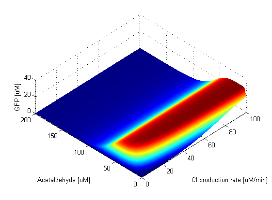
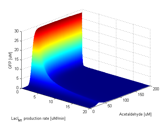
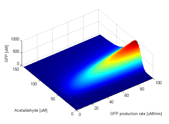
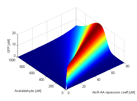
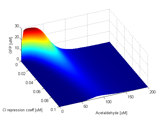
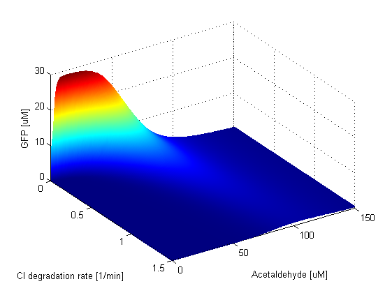
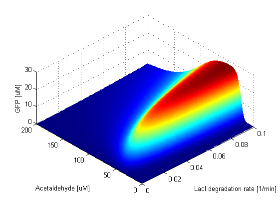
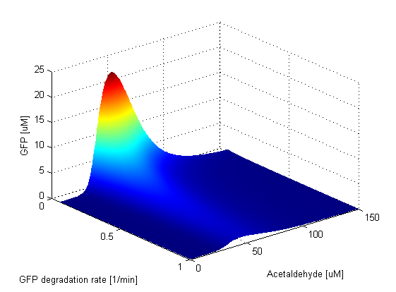
Parameter Sweeps

For the parameters that belong to the band detector module, we explored their parameter spaces to quantify how they affect the features of the GFP band . As we varied each parameter (while keeping the rest constant), we varied also the acetaldehyde input and monitored the GFP output. We analyzed the parameter space only for the model that uses acetaldehyde as an input parameter.

In both models the band is affected in the same way by the parameters of the band detector module. The sensor mechanism can only cause shifts in the band but the band detector module itself is unaffected by the input of the system. The parameter sweeps for the xylene model would therefore be similar to the acetaldehyde model, with differences only for the parameters involved in the sensor mechanism.

In order to speed up the simulations, we used Maple to derive the steady-state formulas for all the relevant species. In this way we were able to obtain the steady-state GFP value simply by knowing the input concentration of Acetaldehyde, without the need to use an ODE solver. Thus we were able to reduce the simulation time from about 30 minutes to under one minute for one parameter sweep.

The following figures show how the band changes with the variation of protein production rates, repression coefficients and degradation rates.

Protein Synthesis Rates

Figure 1: Exploring the parameter space of TetR production rate	Figure 2: Exploring the parameter space of CI production rate
When the TetR production rate is zero, there is no TetR present in the cell, which means that LacI_M1 is not repressed so it is free to block GFP production. This can be seen in the graph, since at this value of TetR production the band is absent. As soon as the production rate becomes non-zero, the band appears. The existence of the GFP band is not affected by the value of the TetR production rate, the band is present and the peak stays at a constant amplitude. TetR production rate only affects the width and position of the band which widens and shifts to higher acetaldehyde values as the production rate increases. When the CI production rate is zero, there is no CI present in the cell, which means that LacI is not repressed, so it is free to block the production of GFP. Thus, the band is absent at this value of CI production rate. After the CI production rate goes above a lower threshold, the band appears. We can observe that above the threshold the GFP band is very robust to the change in CI production rate, maintaining the position and amplitude of the peak at a constant value. The width of the band seems to slightly increase as the CI production rate increases, but at very high values it seems to stay constant.
Figure 3: Exploring the parameter space of LacI production rate	Figure 4: Exploring the parameter space of LacI_M1 production rate
When the LacI production rate is zero, only the low-pass branch of the system is in function. This can be seen in the graph, as GFP is produced if Acetaldehyde has a concentration lower than 100 μM. However, as soon as LacI start being produced the band is formed. When the production rate of LacI gets too high, the amplitude of the band decreases, but the position of the peak and the width stay constant. When the LacI_M1 production rate is zero, only the high-pass branch of the system is in fucntion. This means that GFP is produced only when Acetaldehyde is present and its concentration is higher than a low threshold, which is equal to about 20 μM. When LacI_M1 appears in the cell, the band is formed. Just as in the case of the LacI production rate, the band seems to maintain its width and the position of its peak, but it decreases its amplitude. This is due to the fact that both LacI and LacI_M1 repress GFP production, and if their production rate is high the repression is more efficient.
Figure 5: Exploring the parameter space of GFP production rate
The GFP production rate has an effect only on the amplitude of the band. This is clear from the ODE of the GFP change in time. The amplitude of the GFP is thus directly proportional to the value of the GFP production rate. This can be seen in the graph. When the GFP production rate is zero, naturally no GFP molecules are produced. As soon as the production rate becomes nonzero, the band appears and its amplitude is increasing linearly with the value of the GFP production rate. The width of the band and position of the peak stay fixed.

Repression Coefficients

Figure 6: Exploring the parameter space of AlcR-AA repression coefficient	Figure 7: Exploring the parameter space of TetR repression coefficient
When the AlcR-AA repression coefficient is zero, TetR is always repressed. This in turn means that LacI_M1 is always produced and it represses GFP production. Thus the band is absent. As soon as the AlcR-AA repression coefficient becomes nonzero, the band appears. Since when this value is low, repression of TetR is very efficient, the band is narrow. This can be clearly seen in the graph: the band widens and shifts the position of its peak to higher Acetaldehyde values as the repression becomes weaker. The AlcR-AA repression coefficient influences the lower and upper thresholds which determine where the band is positioned. The amplitude of the GFP band is not affected by the change of this parameter. When the TetR repression coefficient is zero, CI and LacI_M1 are completely repressed, thus LacI is free to repress GFP and the band is absent. Since TetR is produced only when the Acetaldehyde concentration is low, if simultaneously the TetR repression coefficient is low, then GFP is repressed, however for higher Acetaldehyde concentrations GFP is produced. This is why in the graph we notice that for low TetR repression coefficients, above a certain Acetaldehyde concentration there is always GFP present. For high values of the TetR repression coefficient the opposite thing happens. GFP is produced for low Acetaldehyde concentrations because in this case repression of CI and LacI_M1 is weak. Thus the TetR repression coefficient has an impact on the width and position of the band, but again the amplitude remains at the same value.
Figure 8: Exploring the parameter space of CI repression coefficient	Figure 9: Exploring the parameter space of LacI repression coefficient
We observe that the GFP band is sensitive to the CI repression coefficent and appears only for low values of it. CI is responsible for repressing LacI, which in turn represses GFP. If the repression coefficient of CI is zero, LacI will never be produced so GFP is present. For low values of the CI repression coefficient the band will be present because even if there are very few CI molecules in the cell, they will still be able to repress LacI and produce GFP. As the value of the CI repression coefficient gets higher, repression of LacI gets weaker, so GFP is produced less and less. This is visible in the graph, as we can notice that the band is dissapearing for high values of the CI repression coefficient. The LacI repression coefficient direclty affects GFP production since GFP is repressed by LacI and LacI_M1. When this repression coefficient has low values, GFP is always repressed by either LacI or LacI_M1. For intermediate values, the band can be clearly distinguished. For high values of the LacI repression coefficient, the repression of GFP is very weak, so even for high Acetaldehyde concentrations where LacI_M1 should repress GFP, this does not completely happen and we get leaky GFP production.

Protein Degradation Rates

Figure 10: Exploring the parameter space of TetR degradation rate	Figure 11: Exploring the parameter space of CI degradation rate
TetR production is high when the Acetaldehyde concentration is below 20 μM. If the TetR degradation rate is very low, the GFP band appears at higher Acetaldehyde concentrations and it shifts towards lower Acetaldehyde concentration as the TetR degradation rate increases. The amplitude of the band is unaffected however. When the TetR degradation rate is very high, TetR is degraded almost instantly after it is produced, meaning that TetR is almost always absent in the cell. Thus LacI_M1 is free to repress GFP and the band dissapears. The branch that includes CI should repress GFP when the Acetaldehyde concentration is low, that is when TetR concentration is high. When the CI degradation rate is low, CI is able to repress LacI to allow the band to form. However, when the CI degradation rate gets higher, there are too few CI molecules in the cell, and they are not able to repress LacI. This is the reason why at these values of the degradation rate the band is dissapearing.
Figure 12: Exploring the parameter space of LacI degradation rate	Figure 13: Exploring the parameter space of GFP degradation rate
LacI and LacI_M1 direclty repress GFP. We notice that the amplitude of the GFP peak and the bandwidth exhibit positive correlation with respect to the LacI degradation rate. This is due to the fact that as the degradaton rate increases, there are fewer LacI and LacI_M1 molecules in the cell and thus more GFP will be produced. As expected, there is a strong negative correlation between the height and width of the peak and the GFP degradation rate. This is due to the fact that the GFP band can exist only if the GFP molecules are not degraded too quickly.

Coupled parameter variation

With doing the parameter sweeps for individual parameters, we saw how robust our system is with respect to a particular paramter. But in reality, when parameters vary, they usually don't vary alone, but they are coupled (i.e more parameters vary simultaneously). One way to incorporate this fact in our model is to couple the expression rates of the proteins according to the plasmid they are expressed on and vary them together.

Stochastic Simulations

Besides the parameter space search, we performed another type of analysis in order to verify that our system is robust and that it is not bistable. We were especially interested at the GFP band and whether it is always there.

We did stochastic simulations to see how our system reacts to noise and how it responds to perturbations. For a certain acetaldehyde concentration (which gives the peak of the band) we wanted to see how the GFP peak value varies over long time period when we consider stochasticity.

For the stochastic simulations we used the software Dizzy, to which we gave as an input file an SMBL file with the description of our system. Moving from deteministic to stochastic simulations, we had to change several things in the SBML file. For instance, we had to convert all the concentrations into number of molecules (and round them) and also separate the ODEs for the species into ODEs for distinct reaction channels (i.e. separate degradation from activation/repression) etc.

We started with a deterministic simulation to take the deterministic steady states of the species, after 5000 min(the acetaldehyde amount was the one that leads to the maximal GFP value, i.e the peak of the band). Starting from deterministic steady states, we performed a stochastic simulation with Gillespie-direct algorithm for 10000 min in order to get the stochastic steady states. After that, we restarted the stochastic simulation having the stochastic steady state values as our initial and simulated for 100 000 more minutes (storing the GFP values every minute). We collected all the GFP values from the last simulation and plotted them in a histogram (150 bins).

We see in Figure 1 that we obtain a Gaussian distribution of GFP number of molecules at the steady state, with a mean of 23491 molecules and standard deviation of 667 molecules. If we convert this value to concentration we get 19.5046 μM, which is very close to what we obtained deterministically. We see that the system keeps fluctuating -very closely to its steady state, with no large jumps away from it. The fact that the Gaussian distribution is unimodal tells us that our system is monostable. From this analysis we confirmed what we concluded before and that is the robustnes of our system, especially of the GFP band. We can now be sure that for a certain acetaldehyde concentration once the band appears, it won't start fading away.

Sensitivity Analysis

Sensitivity analysis is a technique that studies the change of the output (or any observable) of a certain function with the variation of a certain parameter. It gives us an overview of how sensitive the model is with respect to the parameter, i.e. what the impact of the parameter is. The sensitivity is defined as the partial differential equation of the observable with respect to a certain parameter.

We performed sensitivity analysis with respect to acetaldehyde or xylene. For different input concentrations we monitored the change in the GFP output (dGFP/dAcetaldehyde or dGFP/dXylene).

Figure 14: Sensitivity analysis with respect to acetaldehyde

For the acetaldehyde model, it can be seen from the above figure that the sensitivity is highest when GFP rises. For the peak itself (at [AA] = 1000uM), the sensitivity drops down and then rises again once GFP concentration starts decreasing. This tells us that the GFP concentration level is most sensitive to acetaldehyde at those concentrations where GFP rises and falls.

@@ Line 123: / Line 123: @@
 For the stochastic simulations we used the software Dizzy, to which we gave as an input file an SMBL file with the description of our system. Moving from deteministic to stochastic simulations, we had to change several things in the SBML file. For instance, we had to convert all the concentrations into number of molecules (and round them) and also separate the ODEs for the species into ODEs for distinct reaction channels (i.e. separate degradation from activation/repression) etc.
-We started with a deterministic simulation to take the deterministic steady states of the species, after 5000 min(the acetaldehyde amount was the one that leads to the maximal GFP value, i.e the peak of the band). Starting from deterministic steady states, we performed a stochastic simulation with Gillespie-direct algorithm for 10000 min in order to get the stochastic steady states. After that, we restarted the stochastic simulation having the stochastic steady state values as our initial and simulated for 100 000 more minutes (storing the GFP values every 10th minute). We collected all the GFP values from the last simulation and plotted them in a histogram (150 bins).
+We started with a deterministic simulation to take the deterministic steady states of the species, after 5000 min(the acetaldehyde amount was the one that leads to the maximal GFP value, i.e the peak of the band). Starting from deterministic steady states, we performed a stochastic simulation with Gillespie-direct algorithm for 10000 min in order to get the stochastic steady states. After that, we restarted the stochastic simulation having the stochastic steady state values as our initial and simulated for 100 000 more minutes (storing the GFP values every minute). We collected all the GFP values from the last simulation and plotted them in a histogram (150 bins).
-We see in Figure 1 that we obtain a Gaussian distribution of GFP number of molecules at the steady state, with a mean of 23477 molecules and standard deviation of 648 molecules. If we convert this value to concentration we get 19.4927 &mu;M, which is very close to what we obtained deterministically. We see that the system keeps fluctuating -very closely to its steady state, with no large jumps away from it. The fact that the Gaussian distribution is unimodal tells us that our system is monostable. From this analysis we confirmed what we concluded before and that is the robustnes of our system, especially of the GFP band. We can now be sure that for a certain acetaldehyde concentration once the band appears, it won't start fading away.
+We see in Figure 1 that we obtain a Gaussian distribution of GFP number of molecules at the steady state, with a mean of 23491 molecules and standard deviation of 667 molecules. If we convert this value to concentration we get 19.5046 &mu;M, which is very close to what we obtained deterministically. We see that the system keeps fluctuating -very closely to its steady state, with no large jumps away from it. The fact that the Gaussian distribution is unimodal tells us that our system is monostable. From this analysis we confirmed what we concluded before and that is the robustnes of our system, especially of the GFP band. We can now be sure that for a certain acetaldehyde concentration once the band appears, it won't start fading away.
 |}