Team:ETH Zurich/Modeling/Stochastic
From 2011.igem.org
(→Method) |
(→Method) |
||
| Line 12: | Line 12: | ||
For the stochastic simulations we used the [http://magnet.systemsbiology.net/software/Dizzy/ Dizzy] software, to which we gave as an input an SBML file with the description of our system. Moving from deterministic to stochastic simulations we had to change several things in the SBML file. Firstly, we exported the SBML file to a CMDL format.Next, we converted the species values as well as the production rates and repression coefficients from concetrations (in μM) to numbers of molecules. Since our initial system was described in terms of ODEs, we also had to change this by separating the system into distinct reaction channels (i.e. separate degradation from activation/repression) and specifying the reaction rates. | For the stochastic simulations we used the [http://magnet.systemsbiology.net/software/Dizzy/ Dizzy] software, to which we gave as an input an SBML file with the description of our system. Moving from deterministic to stochastic simulations we had to change several things in the SBML file. Firstly, we exported the SBML file to a CMDL format.Next, we converted the species values as well as the production rates and repression coefficients from concetrations (in μM) to numbers of molecules. Since our initial system was described in terms of ODEs, we also had to change this by separating the system into distinct reaction channels (i.e. separate degradation from activation/repression) and specifying the reaction rates. | ||
<br> <br> | <br> <br> | ||
| - | With the new description of the system, we could start the simulations. For analyzing the robustness of the system, we chose 5 strategic Acetaldehyde concentrations (see Figure 1 | + | With the new description of the system, we could start the simulations. For analyzing the robustness of the system, we chose 5 strategic Acetaldehyde concentrations (see Figure 1), and for each of them we performed stochastic simulations. We selected the following Acetaldehyde concentrations: |
* 0 μM (0 molecules). At this concentration the GFP output should approach 0 μM. | * 0 μM (0 molecules). At this concentration the GFP output should approach 0 μM. | ||
* 25 μM (30110 molecules). At this concentration GFP rises quickly, so it should be very sensitive to noise. | * 25 μM (30110 molecules). At this concentration GFP rises quickly, so it should be very sensitive to noise. | ||
| Line 18: | Line 18: | ||
* 100 μM (120440 molecules). At this concentration GFP is decreasins, so it should be sesnsitive to noise. | * 100 μM (120440 molecules). At this concentration GFP is decreasins, so it should be sesnsitive to noise. | ||
* 300 μM (361320 molecules). At this concentration the GFP output should again approach 0 μM. | * 300 μM (361320 molecules). At this concentration the GFP output should again approach 0 μM. | ||
| - | + | <br> <br> | |
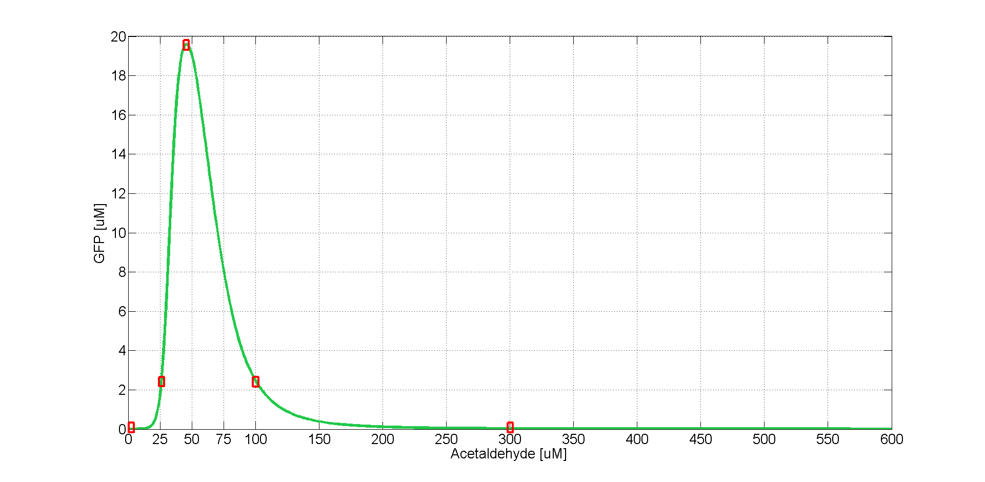
[[File:GFPmlabel.png|thumb|900px|center|'''Figure 1''': GFP versus Acetaldehyde. The red squares denote the 5 Acetaldehyde concentrations for which we simulated the time course of GFP steady state in stochastic mode.]] | [[File:GFPmlabel.png|thumb|900px|center|'''Figure 1''': GFP versus Acetaldehyde. The red squares denote the 5 Acetaldehyde concentrations for which we simulated the time course of GFP steady state in stochastic mode.]] | ||
Revision as of 12:13, 27 October 2011
Stochastic Analysis
Besides the parameter space search, we performed another type of analysis in order to verify that our system is robust and that it is not bistable. We were especially interested in the GFP band, whether it is always present and whether the amount of GFP produced in the cells for different concentrations of Acetaldehyde has large fluctuations. Because gene expression is an intrinsically stochastic process, we performed stochastic simulations to see how our system reacts to noise and how it responds to perturbations.
The following results show that our system is indeed robust and it does not have bifurcations.
Method
For the stochastic simulations we used the [http://magnet.systemsbiology.net/software/Dizzy/ Dizzy] software, to which we gave as an input an SBML file with the description of our system. Moving from deterministic to stochastic simulations we had to change several things in the SBML file. Firstly, we exported the SBML file to a CMDL format.Next, we converted the species values as well as the production rates and repression coefficients from concetrations (in μM) to numbers of molecules. Since our initial system was described in terms of ODEs, we also had to change this by separating the system into distinct reaction channels (i.e. separate degradation from activation/repression) and specifying the reaction rates.
With the new description of the system, we could start the simulations. For analyzing the robustness of the system, we chose 5 strategic Acetaldehyde concentrations (see Figure 1), and for each of them we performed stochastic simulations. We selected the following Acetaldehyde concentrations:
- 0 μM (0 molecules). At this concentration the GFP output should approach 0 μM.
- 25 μM (30110 molecules). At this concentration GFP rises quickly, so it should be very sensitive to noise.
- 46 μM (55402 molecules). This is the concentration that gives the peak GFP value.
- 100 μM (120440 molecules). At this concentration GFP is decreasins, so it should be sesnsitive to noise.
- 300 μM (361320 molecules). At this concentration the GFP output should again approach 0 μM.
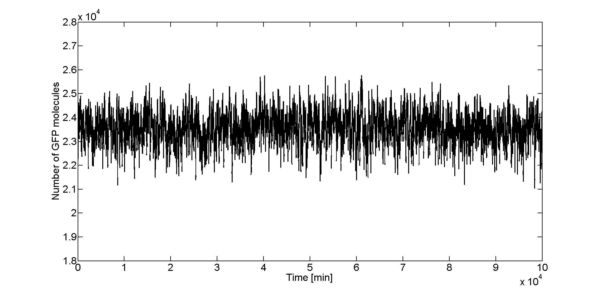
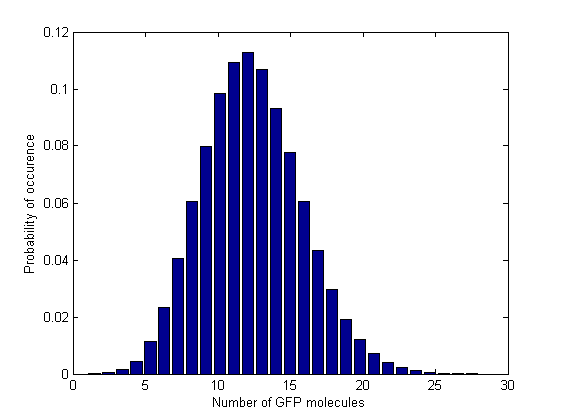
We started with a deterministic simulation to take the deterministic steady states of the species, after 5000 min(the acetaldehyde amount was the one that leads to the maximal GFP value, i.e the peak of the band). Starting from deterministic steady states, we performed a stochastic simulation with Gillespie-direct algorithm for 10000 min in order to get the stochastic steady states. After that, we restarted the stochastic simulation having the stochastic steady state values as our initial and simulated for 100 000 more minutes (storing the GFP values every minute). We collected all the GFP values from the last simulation and plotted them in a histogram (150 bins).
Simulations
|
| |
|
| |
Analysis of Results
Insert overview of page here
 "
"


