 "
"
Team:Grenoble/Projet/Modelling/Deterministic
From 2011.igem.org
Construction of the model
You need MathML supported on your browser to read the equations on this page. However, you can find these equations in the above PDF version.
As a proof of concept, we will consider anhydrotetracycline (aTc) instead of Mercury in our model, and the transcriptional regulator TetR in place of MerR. The TetR system is well characterized in E. coli, which facilitates the modelling. In addition, if the system works well with aTc, it should work as well with Mercury, Copper or lead for example.
In addition, since aTc diffuse freely accross the membrane of the cell, we do not have to take
complex uptake mechanisms into considerations. Mercury is ionized and its entry in the cells
depends on the presence of transporter protein.
So in the following chapter, we are going to use TetR instead of MerR and aTc instead of
Mercury.
The Two levels of Modelling
Our system is divided in two independant system:
- Toggle Switch modelling: To predict in which states bacteria will be on the plate.
- Quorum Sensing and Coloration: To predict where the red line will appear on our device.
The first level of the model will allow us to define the switch conditions in bacteria, depending on the concentrations of pollutant and IPTG. From these results, we could see where the switch zone will appear on the device and therefore, the position of the red line. These parts of the results indicate the range of mercury that can be detected.
The second level will provide us with the red line width, an indicator of the system precision. From these results, we could improve the precision of our device, for instance, by choosing between a device with a continuous bacterial layer and a device with strips containing bacteria. Each strip has a different IPTG concentration, but the same concentration of Mercury.
Two independent levels of modelling which are coupled in order to get a global simulation of the device.
Establishment of the equation
Toggle switch
In a first part, we define a model to caracterize the Toggle Switch part of our genetic network.
In order to get the state of the bacteria, we need to compute the concentration of both
repressors. To obtain these variation, we set up the system of differential equations which governs
the behavior of the Toggle Switch.
- Biological Models
- Mathematical Models
A toggle switch consists of two genes, each coding for a protein that represses the expression of the other gene. This double repression system ensures the basic function of a toggle switch: a bistable system which can be switched from one state to the other by putting, in our example, some IPTG or aTc molecules in the medium.
The biological system we are trying to implement is more complex, on both the biological and physical side. However, the toggle switch model is basically the same. In the study of the toggle switch itself, the system can be reduced to a simple two-state subsystem that we will then use for the rest of our modelling. The toggle switch itself is not influenced by the rest of the system, if we do not consider the RsmA regulatory system that will be modeled at the very end of our work. Thus we will be able to model the toggle switch independently and then build the rest of the model upon this basis.
In a first part, we define a model to caracterize the Toggle Switch part of our genetic network. In order to get the state of the bacteria, we need to compute the concentration of both repressors. To obtain these variation, we set up the system of differential equations which governs the behavior of the Toggle Switch.
$\frac{d[lacI]}{dt} = \frac{k_{pTet}.[pTet]_{tot}}{1 + (\frac{[tetR]}{K_{pTet} + \frac{K_{pTet}.[aTc]}{K_{TetR-aTc}}.})^\gamma} - \delta_{lacI}.[lacI]$
A demonstration of this system of ODE is available in the previous pdf file.
With this ODE’s system, we follow the evolution of the concentration of the two repressors of the toggle switch, TetR and LacI. Which is giving us the state of the bacteria.
Both equations are construct using the same approach. There is a term of production and a term of degradation. Parameters kpLac .[pLac]tot represents the synthesis rate of the promoter pLac. KpLac is the dissociation constant of LacI and pLac. KlacI−IPTG is the dissociation constant of lacI and IPTG. The parameters β and γ traduce the cooperativity of repression, which means the number of repressors bound to the promoter.
We can see from this system, that the rate of variation of repressor TetR is modulated by the concentration of the repressor lacI which inhibits TetR synthesis which itself depens on the IPTG concentration. Reciprocally in the second equation, the variation of lacI depends on TetR which is modulated by aTc.
This indicates that the two equations are coupled. And also that only one repressor could be predominant, as shown later.
These two equations can be easily computed with a differential solver. We can precisely estimate the effects of each parameter.
Establishment of the equation
Quorum sensing
- Mathematical Models
- the production of the Quorum Sensing molecule
- the secretion of the molecule
- the diffusion of the molecule in the medium
- the penetration of the molecule
- the complexation of the molecule with its receptor
- the activation of the coloration
- $[QS_i]$ concentration of the intracellular Quorum Sensing.
- $[QS_e]$ concentration of the extracellular Quorum Sensing.
- $[cinR]$ concentration of the Quorum Sensing receptor.
- $[cinI]$ concentration of the Quorum Sensing producer enzyme.
- $[cinR_{comp}]$ concentration of the complexe cinR-QS.
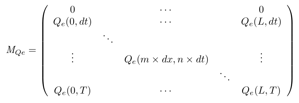
- Definition of the matrix
- On the spatial point of view, we only consider the x dimension, as the IPTG gradient will be only evolving along this dimension. Thus we consider the state of our cells is the same along the width of our plate.
- With this Matrix, and after computation of all the terms, we can get the entire behaviour of CinI, CinR, QS inside and outside the cells.
- The first line of the Matrix equals 0. These are the initial conditions we set to 0 at time t = 0s.
- On the borders of the plate (x = 0 and x = L) the model used has to be different, limit conditions will be set.
- Of course, Qi, CinI and CinR matrices will be similarly implemented.
- Discretization of the equation
In a second part, we define a model able to caracterize the quorum sensing part of our genetic network perfomed by quorum sensing genes.
Our work mainly refers to the models set up by the 2007 iGEM Bangalore team. On the basis of their work we set up models adapted to our own system. For these reasons we strongly recommend getting familiar with the works of the 2007 Bangalore team for an easier understanding of the models we used.
The main difference between our models is that their model is designed for a whole medium, in which the concentrations of quorum sensing molecules are considered for a whole fixed volume of a medium. Our system, however, is supposed to describe the spatial diffusion of quorum sensing molecules as well, and therefore needs to be designed for an infinitesimal volume of medium containing bacteries and outside medium. A few other differences exist between our model and theirs, mainly due to the fact that the system we intend to describe is made of other different parts. For example the production rate of our Quorum Sensing enzymes are directly linked to the previously described toggle switch model.
For these reasons we strongly recommend getting familiar with the works of the 2007 Bangalore team for an easier understanding of the models we used.
In a second part, we define a model able to caracterize the quorum sensing part of our genetic network
perfomed by quorum sensing genes.
At the boundary, quorum sensing molecules produced by secretory bacteria diffuse and enter in the receving bacteria.
In order to well characterize the quorum sensing part, we need to well understand the mecanism.

According to the figure, several steps must be taken into account:
To model these mecanisms, we need to follow the evolution of the following quantities
Based on the Bangalore 2007 iGEM team, we get the following system of equations:
$\frac{d[QS_e]}{dt} = \rho v_c\eta([QS_i]-[QS_e])-\delta_{QSe} [QS_e] + D_{diff}\frac{\partial^2 [QS_e]}{\partial x^2}$
$\frac{d[cinR_{free}]}{dt} = \frac{k_{pLac}.[pLac]_{tot}}{1 + (\frac{[lacI_{total}]}{K_{pLac} + \frac{K_{pLac}.[IPTG]}{K_{lacI-IPTG}}.})^\beta} - \delta_{cinR}[cinR_{free}] - V_{complexation}$
$\frac{[cinR_{comp}]}{} = K_{comp}([cinR_{free}].[QS_i])$
In the first equation, expressing the evolution of intracellular Quorum Sensing, 3 terms are involved: $[QS_e]-[QS_i]$ the diffusion through the membrane, $\delta_{QSi} [QS_i]$ the degradation and $k_{QS-production}'[cinI]$ the production of Quorum Sensing by the enzyme cinI. In the second equation, expressing the evolution of extracellular Quorum Sensing, there is no production term, but a spatial diffusion term $D_{diff}\frac{\partial^2 [QS_e]}{\partial x^2}$.
To get the concentration of cinI and cinR, we used the toggle switch modelling. In fact, cinI is on the pathway of lacI and cinR on the pathway of TetR and their evolution follow the same equations. But we need to consider the complexation of cinR protein and Quorum Sensing molecule which is expressing by the term $V_{complexation}$ in the cinR equation. \[V_{complexation} = K_{comp}[QS_i][CinR_{free}]\] with $K_{comp}$ the affinity constant of AHL for cinR.
In order to simplify the model, we considered that the complexation is totally done and depends only on $[cinR]$ and $[QS_i]$.
To solve this set of equation, we couldn't use an ODE's matlab solver because equations were derived both in time and space. That's why, we needed to use the finite differences method. For this, we build a matrix based on Taylor's series discretization.
To solve this set of equations we have to use a matrix that will describe our system in both space and time. for example for the QS molecule outside of the cell :
$M_{QSe}(m+1,n+1) = [QS_e](x + dx,t+dt)$
With our continuous equations set, we want to obtain discrete definition of each of the matrices. The interdepen- dancies of the equations imply that the computation of the matrices will be performed on the entire CinI matrix first, then each line of the Qi and Qe matrices will be computed alternatively. Finally CinR matrix computation will be performed.
Parallel computation of all the matrices without proper control is not possible indeed, as the terms of Qi matrix will depend on the Qe terms of the preceding line (and vice-versa). Discretization is obtained with first order taylor series :
$ M_{QSe}(m,n+1) =\Delta t ( D_{m} + D_{diff} \frac{M_{QSe}(m+1,n) - 2 M_{QSe}(m,n) + M_{QSe}(m-1,n)}{\Delta x^2}) + M_{QSe}(m,n) $
$ with D_{m} =\rho v_c \eta .M_{QSi}(m,n) - M_{QSe}(m,n)(\delta_{QSe} + \rho v_c \eta) $
$ M_{CinR_{free}}(m,n+1) = \Delta t (\frac{k_{pTet}[P_{Tet total}]}{1+ (\frac{[TetR]}{K_{pTet}(1+\frac{[aTc]}{K_{TetR - aTc}})})^{n_{pTet}}} - M_{CinR_{free}}(m,n)(\delta_{CinR} - k_{comp}.M_{Qi}(m,n))) + M_{CinR_{free}}(m,n)$
With these discrete equations the 4 matrices can be computed through simple calculation loops over each line. The CinI matrix does not depend on space dimension, it is then possible to compute it without discretization with a differential solver.
Our algorithms
In the MATLAB archive that can be found here containing our matlab scripts for deterministic modelling (file Deterministic_archive.tar.gz) you can launch an ODE based simulation (see our ODEs in the two previous sections) with the file biosenseur1Dmain.m.
Several dialog boxes will pop up to enter the specificities of the simulation : (physical specificities of the device, chemical species concentrations and IPTG gradient )
At the end of the simulation you obtain 3 matrices named M_stock, M_QS and M_comp containing the concentrations in each protein species at each time point and on each physical point of the plate. We wrote three MATLAB scripts that display the concentration in proteins dynamically that you can call with DynamicplottingTS, DynamicplottingQS and DynamicplottingCP. For a good understanding of the models and of our results we also wrote a script to illustrate the coloration of our plate through time according to our models named Imageshow.m.