Team:USTC-Software/parameter
From 2011.igem.org
 USTC-Software
Parameter Analysis
We tried on the following prospect and finished the test code with Matlab (ready and eager to implement the test codes into Lachesis)
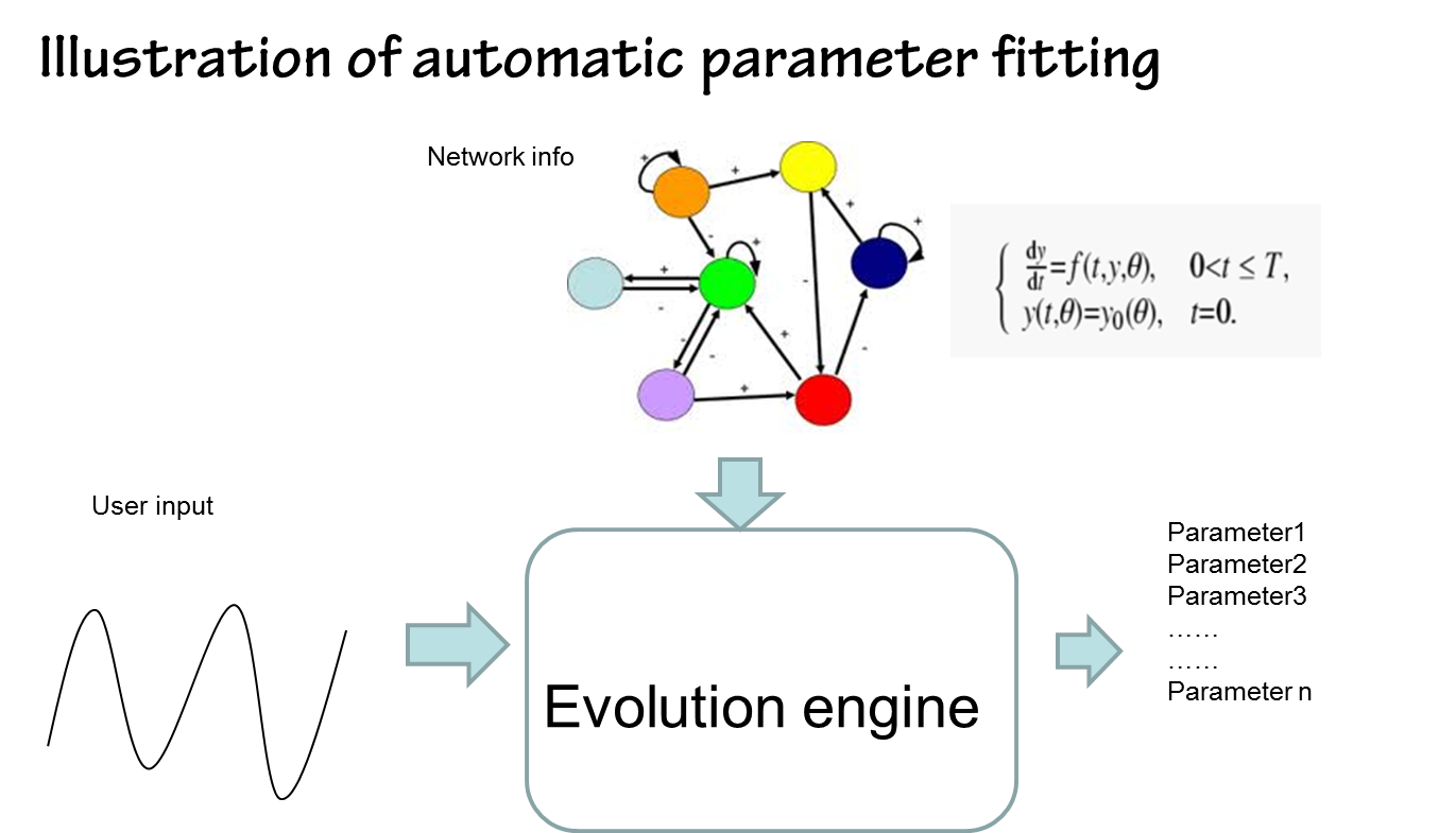
* Automatic parameterfitting, adjustment, and estimation with a given mathematical structure: User selects the standard or criteria according to wet LAB data or just describe what they want to be output. Minimize the cost function using simulated annealing.
* Evaluate a design with user input and pre-defined criteria from different aspect: Analyze the sensitivity and robustness of a given network using random sampling and pca analysis(principle component analysis).
Part1 Parameter section:
1.1 Background
Almost ideal tools that already exist in electronics: User provide the part’s name, the software fetch the standard model and its associated parameter, and return a complete mathematical model with all the parameters known (for instance, the PROTEL-software can easily get the released device from the NI company with all the response parameters standardized from a device library).
But currently, the knowledge and cognition level of synthetic biology do not support this: Most parts do not have a standard model associated with it. Some parameters of the parts haven’t been measured yet. Some parts with quantitative parameter values, which are highly context dependent, are hard to transfer with defined parameters across different hosts.
1.2 More consideration
Why do we try automatic parameter fitting(or estimation, adjustment)?
• If it’s a big network with too many parameters undefined, it would get the user exhausted adjusting all the empty parameters by hand according to his/her experience and web resource. Network generated by rule based modeling is ordinarily large
• Compared to manually parameter adjustment, in silicon auto parameter adjustment is more convenient.It gives an estimation of the interest parameter value according to wet lab data, thus free the user from spending too much time on estimating a good parameter.
1.3
We adopted a demo from a Tinkercell tutorial website on implementing a simple repressilator. After the network is generated by hand, the parameters are left behind to the user to adjust by themselves. But as you can see from the following figures, the process is tough and time consuming. (more snapshots of the process of manual parameter fitting are eliminated )
<--


………………(more trial and error)
 !-->
[[File:manual parameter fitting.png|500px]]
The four figures above show a difficult parameter adjustment process by hand.
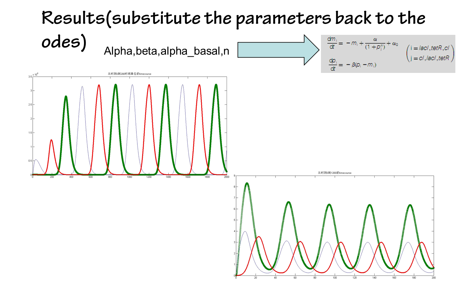
By contrast, parameters estimated by our approach in silicon can be done in a timely fashion. It’s fast and convenient(see figure below)
 the results are shown below(we choose the classical repressilator as an example)

1.4 Algorithm
Particle swarm optimization (PSO) Algorithm
History
Particle swarm optimization (PSO) is a population based stochastic optimization technique developed by Dr. Eberhart and Dr. Kennedy in 1995, inspired by social behavior of bird flocking or fish schooling. The particle swarm concept originated as a simulation of simplified social system. The original intent was to graphically simulate the choreography of bird of a bird block or fish school. However, it was found that particle swarm model can be used as an optimizer.
Algorithm introduction
Each particle keeps track of its coordinates in the problem space which are associated with the best solution (fitness) it has achieved so far. (The fitness value is also stored.) This value is called pbest. Another "best" value that is tracked by the particle swarm optimizer is the best value, obtained so far by any particle in the neighbors of the particle. This location is called lbest. when a particle takes all the population as its topological neighbors, the best value is a global best and is called gbest.
The particle swarm optimization concept consists of, at each time step, changing the velocity of (accelerating) each particle toward its pbest and lbest locations (local version of PSO). Acceleration is weighted by a random term, with separate random numbers being generated for acceleration toward pbest and lbest locations.

Application
PSO has been successfully applied in many research and application areas. It is demonstrated that PSO gets better results in a faster, cheaper way compared with other methods.
Simulated Annealing(SA) Algorithm
Simulated annealing (SA) is a generic probabilistic metaheuristic for the global optimization problem of locating a good approximation to the global optimum of a given function in a large search space. It is often used when the search space is discrete (e.g., all tours that visit a given set of cities). For certain problems, simulated annealing may be more efficient than exhaustive enumeration — provided that the goal is merely to find an acceptably good solution in a fixed amount of time, rather than the best possible solution.
Principle of the algorithm
In the simulated annealing (SA) method, each point s of the search space is analogous to a state of some physical system, and the function E(s) to be minimized is analogous to the internal energy of the system in that state. The goal is to bring the system, from an arbitrary initial state, to a state with the minimum possible energy.
Steps
At each step, the SA heuristic considers some neighbouring state s' of the current state s, and probabilistically decides between moving the system to state s' or staying in state s. These probabilities ultimately lead the system to move to states of lower energy. Typically this step is repeated until the system reaches a state that is good enough for the application, or until a given computation budget has been exhausted.
State transition
The neighbours of a state are new states of the problem that are produced after altering the given state in some particular way. For example, in the traveling salesman problem, each state is typically defined as a particular permutation of the cities to be visited. The neighbours of some particular permutation are the permutations that are produced for example by interchanging a pair of adjacent cities. The action taken to alter the solution in order to find neighbouring solutions is called "move" and different "moves" give different neighbours. These moves usually result in minimal alterations of the solution, as the previous example depicts, in order to help an algorithm to optimize the solution to the maximum extent and also to retain the already optimum parts of the solution and affect only the suboptimum parts. In the previous example, the parts of the solution are the parts of the tour.
Probability function of the state transition
The probability of making the transition from the current state s to a candidate new state s' is specified by an acceptance probability function P(e,e',T), that depends on the energies e = E(s) and e' = E(s') of the two states, and on a global time-varying parameter T called the temperature. States with a smaller energy are better than those with a greater energy. The probability function P must be positive even when e' is greater than e. This feature prevents the method from becoming stuck at a local minimum that is worse than the global one.

Part2 Assessment section:
2.1
Why do we try to evaluate a design with sensitivity and robustness analysis?
• Computer descriptions of biological mechanisms are by necessity,very simplified.
• The biology system is so complex that current mathematical description is far from accurate
• Parameters of biological parts are context dependent and some may vary drastically when host cell or environment change
• Noise come from various sources and can drastically influence the performance of a circuit
• Things that can be implemented through ode parameter adjustment might not necessarily be observed in real experiment.
• If the parameter range is slim at the working region, then most probably the desired phenomena will never be observed in wet experiment
• If we get the most sensitive parameter, we probably know what to do to refine a circuit to quick tune it to a desired behavior or just try to keep that most sensitive parameter as constant as possible.
Part3 Model reduction and network modulation (havn’t done yet)
Below is an aflow chart that demonstrates the whole process:

 "
"
