Team:Paris Bettencourt/Modeling
From 2011.igem.org

Contents |
Modeling
What is modeling in synthetic biology?
Synthetic biology relies heavily on genetic constructs designed to perform a specific task. In order to predict the behaviour of such systems, we need to be able to model it. Knowing in advance how well or how poorly a construct will work can help us during the genetic design phase or when we need to prepare our experiments. We need to describe the future reactions of our system is to create a mathematical model of it.
The bible for synthetic biology modeling is Uri Alon's book An Introduction to Systems Biology: Design Principles of Biological Circuits. Most of our models are based on his approach to biological circuits. We are now going to explain quickly what is the basic structure behind our simulations.
The gene geneX is responsible for the production of the corresponding protein X. The promoter pX controlling the expression geneX can be:
- A constitutive promoter, geneX is activated whatever the conditions
- Positively regulated, geneX is more active when an inducer is present
- Negatively regulated, geneX is less active when an repressor is present
INSERT IMAGE HERE
The inducer or repressor can be another protein or even the product itself. In the latter case, the gene is auto-regulated, wether positively or negatively. To begin, let's assume pX is a constitutive promoter for now. We will make another simplification by taking into account the translation step and assuming that the gene "directly" produces protein X.
We will know take a look at the parameters involved in modeling this network.
X is the concentration of protein X alpha is the expression rate of protein X (mol.s^-1). It mainly depends on the constitutive promoter. delta_dil is the dilution rate, due to cell division (s^-1) delta_deg is the degradation rate of protein X
The equation and solution modeling the behaviour of this system are the following:
INSERT IMAGE HERE (initial conditions zero)
Now, let's assume that pX is auto-regulated, either positively or negatively. We need to introduce a couple of new parameters.
K is the dissociation constant, representing the binding of a inducer/repressor to the promoter n is the Hill coefficient of the function
The equations and solutions are now:
INSERT IMAGE HERE (initial conditions zero, parameters noted)
You will note that the regulation is modeled as a Hill function. This type of functioncan help us model most of the regulation that takes place in a genetic network.
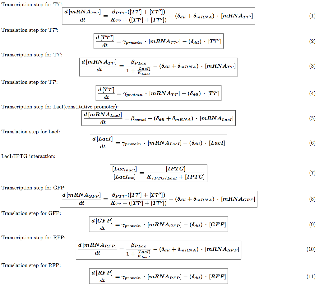
Of course most genetic networks are more complex than simply auto-regulated nodes. The product of one gene can regulated the activation of another which in turn inhibits a third, etc. By coupling this kind of equations together, we achieved modeling most of our genetic networks pretty easily.
Our hypothesis
Direct observation
Characterization
T7 system
tRNA_amber system
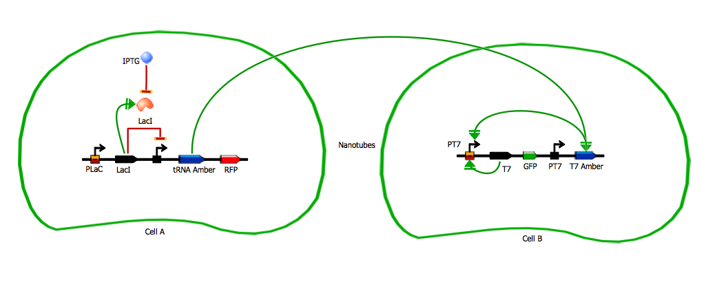
The amber suppressor tRNA diffusion. The idea of the system is to pass tRNA amber molecules through the nanotubes. At every moment of time in the receiver cell there is a certain amount of transcribed mRNA-T7 among the others mRNA. The behavior of tRNA amber that arrived in a receiver cell is random, so in order to describe its interaction with mRNA-T7 and its further translation we can reason in terms of probability.
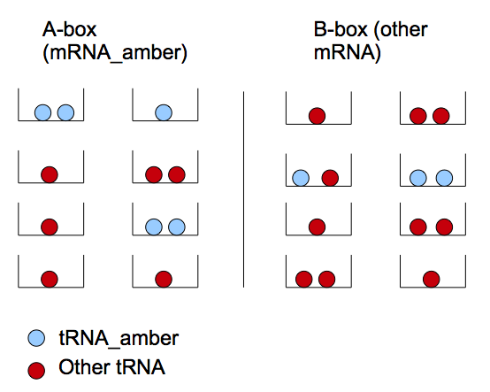
We can reason in two steps : first a tRNA amber molecule gets close to a mRNA molecule. Then, it binds it's anti-codon with a codon of the mRNA. This reasoning is similar to the problem of boxes and balls. There are two types of boxes: 'a' of the first type and 'b' of the second (which corresponds to the set of mRNA-T7 and mRNA-non-T7), and there are 't' balls(tRNA amber). All the balls are randomly distributed in the boxes. If there are two or more balls in some box of the first type (two or more tRNA amber per mRNA-T7) then a T7 molecule will be produced with a chance P_0.
We have defined two models for this system which both rely on the following assumptions :
- Each mRNA is defined as a 'box'
- All the tRNA molecules are uniformly distributed in the boxes.
- The number of tRNA_amber diffused through the nanotubes is much more smaller than the one of the mRNA. Thus the chance that three or more tRNA amber will "find" one mRNA-T7 is negligible comparing to the one of two tRNA amber (finding a mRNA-T7). In our model we will consider that at one moment of time each mRNA interacts with 0, 1 or 2 tRNA ambers.
- The tRNA_amber placed in a correct box are always used
Distribution of tRNA_amber in mRNA populations
We have defined two models for this system which both rely on the following assumptions :
- Each mRNA is defined as a 'box'
- All the tRNA molecules are uniformly distributed in the boxes.
- The number of tRNA_amber diffused through the nanotubes is much more smaller than the one of the mRNA. Thus the chance that three or more tRNA amber will "find" one mRNA-T7 is negligible comparing to the one of two tRNA amber (finding a mRNA-T7). In our model we will consider that at one moment of time each mRNA interacts with 0, 1 or 2 tRNA ambers.
- The tRNA_amber placed in a correct box are always used
Let's define two types of boxes: mRNA_amber ('A') and other type of mRNA ('B'). We note the mRNA_amber producing T7 as mRNA*_amber. The latter appears if we have two tRNA_amber in one box. This model treats the repartition of tRNA_amber in the different boxes.
We note P(x) the probability of having x A-boxes containing two tRNA_amber. Thus P(x=1) corresponds to the probability of finding a couple of tRNA_amber in an A-box, thus to produce x T7 molecules. 't' is the number of tRNA_amber in the cell.
We note:
- P(x=1)= (probability that 2 balls choose A-boxes) * (probability that these 2 balls choose the same A-box) + (probability that 3 balls choose A boxes) * (probability that 2 balls out of 3 choose the same A-box and the third doesn't) + ... + (probability that t balls choose an A-box) * (probability that 2 of these t balls choose the same A-box and the rest don't).
- P(x=2)= (probability that 4 balls choose A-boxes) * (probability that these 4 balls choose 2 A-boxes, one A-box per pair of balls) + (probability that 5 balls choose A-boxes) * (probability that 4 balls out of 5 choose 2 A-boxes, one A-box per pair of balls and the fifth doesn't) + ... + (probability that t balls choose A-boxes) * (probability that 4 out of these t balls choose [t/2] A-boxes, one A-box per pair of balls and the rest don't).
- ...
- P(x=i)= (probability that 2i balls choose A-boxes) * (probability that these 2i balls choose i A-boxes, one A-box per pair of balls) + (probability that (2i + 1) balls choose A-boxes) * (probability that 2i balls out of (2i + 1) choose i A-boxes, one A-box per pair of balls and the rest don't) + ... + (probability that t balls choose A-boxes) * (probability that 2i out of these t balls choose [t/2] A-boxes, one A-box per pair of balls and the rest don't).
Hence:
Master/Slave
Bi-directional communication
Brownian motion and diffusion
A significant part of our designs relies on diffusion of very few molecules activating the amplification and reporter systems. For instance, we know that in the T7 design, we need less than ten T7 RNA polymerases to trigger the amplification. Knowing how a molecule moves in a cell just after its transport through nanotubes was necessary. To model this kind of behaviour we had to look into the mechanisms of diffusion for single molecules in a cell. This meant studying the motions of diffusion.
Please note that we are not talking here about the movement of molecules inside the nanotubes, which requires other types of modeling.
Diffusion without boundary conditions
The first step was to study the general principle of diffusion and to apply them to a single molecule. We expected to estimate the order of magnitude for diffusion time of molecules with this model, not to have a precise understanding of the movement of molecules in a cell. Most of our experimental designs rely on time measurement to characterize the nanotubes, it was therefore crucial to see if diffusion time could add a significant delay to the response of receiver cells.
The principle of this first model is quite simple. We use the statistical diffusion equation with a new normalisation constant so that it describes the behaviour of one molecule. Rather than obtaining a concentration field, we end up with a distribution of the density of probability to find the molecule at a certain position and a certain time. We did not use any kind of boundary conditions, we therefore only model the "movements" of one molecule floating in an infinite water medium.
The equation of diffusion is the following:
Where c is the concentration of particles in the cell, function of <math>\vec{x}</math> (position) and t (time). D is the diffusion coefficient.
The solution for such an equation is:
The star * represents the convolution of the two functions. The first part represents the initial conditions which are in our case a Dirac function centered on the origin of space (there is only one molecule at (0,0,0) at t=0). the second part of this solution is the so-called fundamental solution.
 "
"


