Team:Groningen/modeling simulation engine
From 2011.igem.org
| Line 15: | Line 15: | ||
Using these four types of factors we can generate new models states. By saving every model state we can plot the behavior of our system in an easy and readable way. | Using these four types of factors we can generate new models states. By saving every model state we can plot the behavior of our system in an easy and readable way. | ||
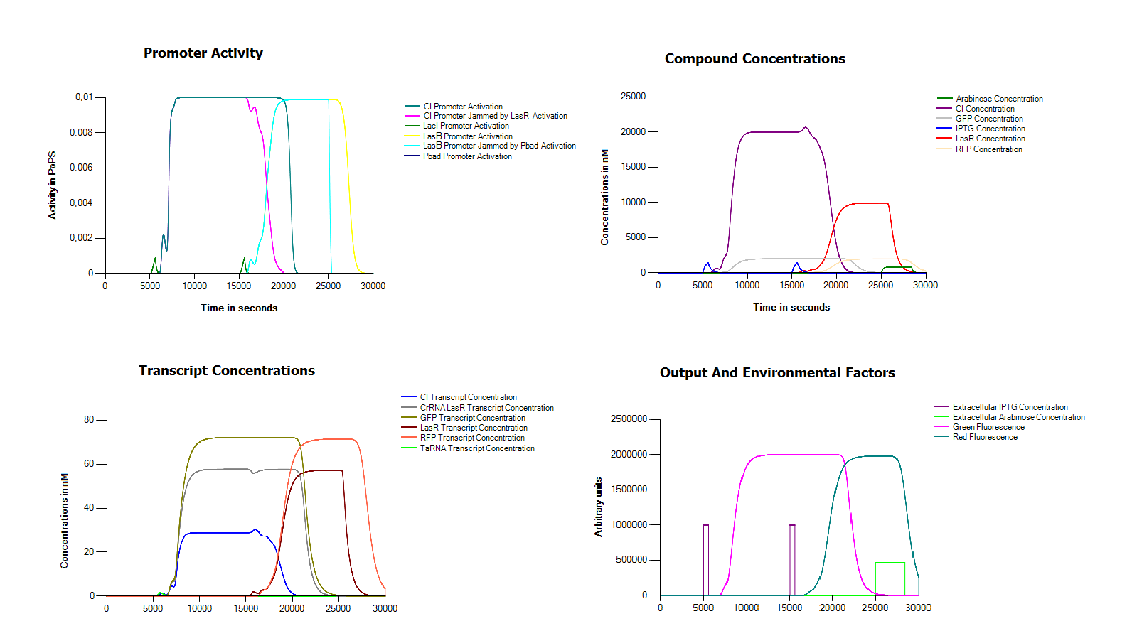
| - | [[File: | + | [[File:Groningen2011FullSimulation.png|thumb|centre|600px|This figure shows a simulation of our full model. Each of the four plotting area's contains information on a different type of factor]] |
| - | + | ||
==Modularity== | ==Modularity== | ||
Latest revision as of 22:19, 21 September 2011
The Cumulus simulation engine
Cumulus uses an internal single cell simulation engine to evaluate parameter settings. The simulation engine is a simple temporal integration over a collection of differential equations. As an input it takes a model of the cell to simulate, some starting conditions, and the input data relating to controlled environmental factors. The timescale we use is seconds since this seems a good middle ground that allows us to characterize the processes we are interested in typically the effects of reporters such as GFP. All faster processes such as diffusion of compound through the cell or the binding of induction factors to operating regions are assumed to occur instantaneously between time steps. Slower processes such as transcription and translation delays are explicitly modeled. The reason we do not allow the use of variable timescales is that these can yield numerically different solutions for the same data. This would break the functionality of Cumulus to compare between models. Hence we decided to maintain consistency within the context of our modeling tool.
The model
For our model we use a deterministic set of differential equations (ODE's and PDE's). All these act on the current model state to compute the next state of the model. This state represents all the important characteristics in a cell which we refer to as factors. However, if need be one could access previous states to facilitate complex temporal progressions such as delays emerging from transcriptions and translations. Also we can save this entire history for any factor so examining in retrospect is possible.
We distinguish four types of factors:
- Promoter activation: Measured in polymerase bindings per second, for instance the activation of a LacI promoter
- Transcript concentrations: Measured in nanomole per liter, for instance the concentration of an RNA molecule coding for cI.
- Compound concentrations: Measured in nanomole per liter, for instance the concentration of an GFP molecule.
- Environmental factors: Measured in different units, for instance temperature or light exposure.
Using these four types of factors we can generate new models states. By saving every model state we can plot the behavior of our system in an easy and readable way.
Modularity
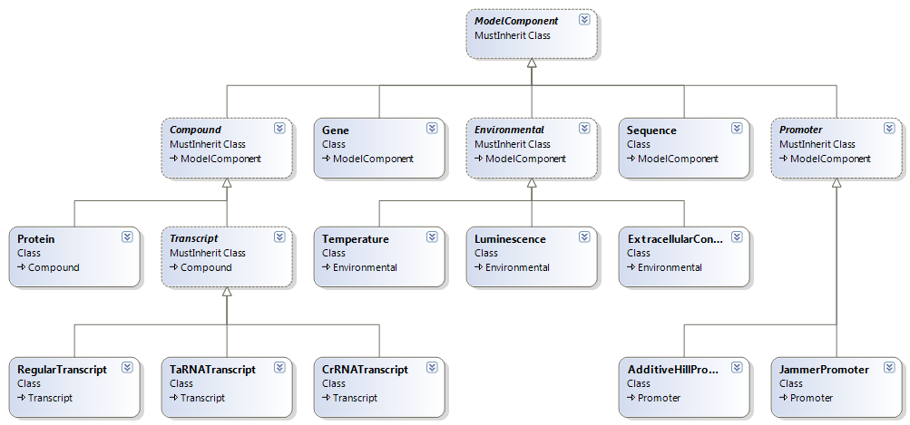
The Cumulus simulation engine is a system of modular object oriented design. Therefore adding new components can be done in a matter of minutes. We only implemented the components we needed for our own system and some test constructs, but the potential for extension is very real. At the moment the simulators biggest constrains are a lack of noise modeling and multicellular support.
- ModelComponent: The abstract base class of all model components. All ModelComponents have a name.
- Compound: The abstract base class of all the stuff floating around inside the cell. Compounds all have a concentration which is registered as nanomoles for every timestep.
- Protein: The class we used for everything that is a compound but not a transcript. Proteins have a concentration decay rate over time, which covers degradation as well as dilution because of cell growth. We used this class not only for proteins but also for smaller molecules that we assumed shared this behavior (such as arabinose or IPTG).
- Transcript: The abstract base class for all transcripts. Treated as everything that is a direct result of a transcription process. Every Transcript has a concentration decay rate. It has several subclasses that express the different types of transcripts we modeled.
- Regular Transcript: This is a transcript that moves on to translation. It has a ribosome binding site strength and a halflife.
- taRNA Transcript: A small transcript that binds to a crRNA transcript top release its ribosome binding site. It has an halflife but no ribosome binding affinity.
- crRNA Transcript: The crRNA is made by wrapping an other construct in this modeling component and adding the reference to a taRNA Transcript. The concentration of the wrapped construct is increased by the crRNA binding to the taRNA transcript. The binding reducing both its own concentration and that of the taRNA in equal amounts and increasing the concentration of the internal transcript by the same amount. For this reaction we assumed the mass action law.
- Gene: Genes are simple components that code for a single protein. They Exist as a abstractionlayer between proteins and the transcript that codes for them.
- Environmental: This abstract base class is the superclass of all modeling components that can not be modified by the cell. They typically contain input and output components.
- Luminescence: An environmental for converting fluorescent molecule concentrations into measurement data. It is initialized with a background an a multiplier but these are not parameters since they are not part of the cell's biological functioning.
- Temperature: An environmental for making temperature input data, it contains functions for making coldshock time series.
- Extracellular Concentration: An environmental for extracellular concentration such as arbinose or IPTG. We assume they slowly diffuse into the cells in the medium. In the future this could further be extended with modelling components that model active transport.
- Promoter: An abstract base class of all promoters. It holds an activation value.
- Additive Hill Promoter: A model of a promoter that can be induced via hill kinetics. It has four parameters that each influence the activation curve of the promoter.
- Jammed Promoter: Our way of modeling the jammers by creating a meta promoter that takes two other promoters as its input. The activity of the meta promoter is calculated by subtracting the activity of the reverse promoter multiplied by some factor from the activity of the forward promoter. This multiplication factor is a parameter of the Jammed Promoter.
 "
"


