Team:UT-Tokyo/Data/Modeling/Model01
From 2011.igem.org
| Line 1: | Line 1: | ||
| - | {{:Team:UT-Tokyo/Templates/BeginContent|fullpagename=Team:UT-Tokyo/Data/Modeling/ | + | {{:Team:UT-Tokyo/Templates/BeginContent|fullpagename=Team:UT-Tokyo/Data/Modeling/Model02|subpagename=Model02}} |
| - | = | + | =Model2: A simple model for E.coli chemotaxis= |
=Aim= | =Aim= | ||
| - | + | We tried to derive a simple relationship between Asp concentration and E.coli chemotaxis so that | |
| - | + | it become possible to simulate macroscopic (n~10<html><sup>8</sup></html>) E.coli-colony chemotactic behavior in the entire simulation. | |
| - | + | ||
| + | =Background= | ||
| + | SPECS <html><sup class="ref">[1]</sup></html> is one of the model simulating E.coli chemotactic behavior. | ||
| + | It considers internal condition of E.coli (receptor methylation etc) so it is a relatively strict taxis model. It is suitable for semi-macroscopic simulation which has around ten thousand E.coli and the timescale is within a hour. | ||
| + | For our system, however, it takes too much time to replicate entire system, because the system includes much more E.coli(about one hundred of million) and the time scale is relatively long (a few days). | ||
| + | Therefore we devised a new model based on SPECS which requires less calculation amount. | ||
=Method= | =Method= | ||
| - | We | + | We approximated chemotactic motion of E.coli groups into two factors, that is, parallel translation and diffusion. |
| + | Let 'V' represents a parallel translation velocity, 'D' represents a diffusion coefficient of E.coli groups and 'A' represents L-Asp concentration. | ||
| + | E.coli can detect A and its gradient ∇A. | ||
| + | They have an internal circuit to translate these signal into motions of their flagellum and try to run toward Asp-richer region. | ||
| + | So we thought V and D could be represented as a functions of A and ∇A. | ||
| + | And then we used SPECS model to derive these functions. | ||
| - | + | Here we introduce SPECS briefly. | |
| + | An E.coli belongs to one of two mobile states: "Run" and "Tumble". | ||
| + | Run state indicates that E.coli goes straight until the state changes. | ||
| + | Tumble state indicates that E.coli is changing its direction and doesn't move around. | ||
| + | E.coli changes its state "Run" to "Tumble" with probability P<html><sub>rt</sub></html> [1/sec]. | ||
| + | "Tumble" to "Run" with P<html><sub>tr</sub></html> [1/sec]. | ||
| + | These probability depend on the E.coli internal state. | ||
| + | The internal state is represented as two variables: "a" and "m". | ||
| + | "a" indicates its kinase activity and "m" represents its receptor's methylation level. | ||
| + | They vary depending on L-Asp concentration. | ||
| + | In addition, SPECS concern the Brownian fluctuation. | ||
| + | From these modeling, SPECS can replicate the internal circuit of E.coli which translates Asp concentration distribution into its mobile state. | ||
| - | + | We processed Monte Carlo simulation for 20000 E.coli which behavior was based on SPECS in some different Asp concentration and its gradient strength. The shape of the Asp gradient we used were exponential. | |
| - | We | + | |
| - | + | [[File:utt_m2_eqn1.png]] | |
| - | + | ||
| - | + | We approximated E.coli movement as the combination of parallel translation and diffusion. | |
| + | We recorded the time course of average position <x> and root-mean-square \<x^2> and then | ||
| + | calculated average velocity | ||
| - | + | [[File:utt_m2_eqn2.png]] | |
| - | + | ||
| - | + | and the diffusion constant. | |
| + | |||
| + | [[File:utt_m2_eqn3.png]] | ||
| + | |||
| + | We derived the relationship between | ||
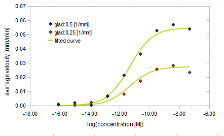
| + | * Asp concentration and average velocity of E.coli | ||
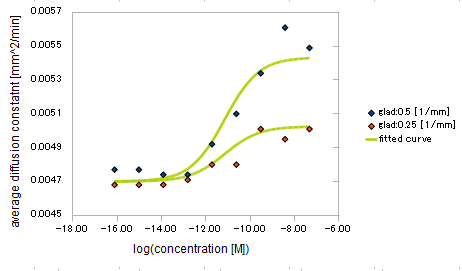
| + | * Asp concentration and diffusion constant of E.coli | ||
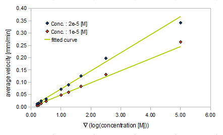
| + | * gradient of Asp concentration and average velocity of E.coli | ||
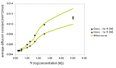
| + | * gradient of Asp concentration and diffusion constant of E.coli | ||
| + | Finally we fitted approximated curve (represented as functions of A and ∇A) to these data so that we could use these functions in the entire simulation. | ||
=Result= | =Result= | ||
| - | + | ||
| - | {{:Team:UT-Tokyo/Templates/Image|file= | + | {{:Team:UT-Tokyo/Templates/Image|file=utt_m2_fig1.png|caption=Figure 1. relationship between Asp conc. and avg. velocity}} |
| + | {{:Team:UT-Tokyo/Templates/Image|file=utt_m2_fig2.png|caption=Figure 2. relationship between gradient of Asp conc. and avg. velocity}} | ||
| + | {{:Team:UT-Tokyo/Templates/Image|file=utt_m2_fig3.png|caption=Figure 3. relationship between Asp conc. and diffusion coef}} | ||
| + | {{:Team:UT-Tokyo/Templates/Image|file=utt_m2_fig4.png|caption=Figure 4. relationship between gradient of Asp conc. and diffusion coef}} | ||
| + | |||
| + | The fitted curves are represented by following equation. | ||
| + | |||
| + | [[File:utt_m2_eqn4.png]] | ||
| + | |||
| + | [[File:utt_m2_eqn5.png]] | ||
<html> | <html> | ||
| Line 32: | Line 71: | ||
<div id="references"> | <div id="references"> | ||
<ul> | <ul> | ||
| - | <li id="ref_1">[1] | + | <li id="ref_1">[1] Jiang L, Ouyang Q, Tu Y (2010) Quantitative Modeling of Escherichia coli Chemotactic Motion in Environments Varying in Space and Time. PLoS Comput Biol 6(4): e1000735. doi:10.1371/journal.pcbi.1000735</li> |
| - | + | ||
</ul> | </ul> | ||
</div> | </div> | ||
</html> | </html> | ||
{{:Team:UT-Tokyo/Templates/EndContent}} | {{:Team:UT-Tokyo/Templates/EndContent}} | ||
Revision as of 19:08, 5 October 2011
Model02

iGEM UT-Tokyo
Model2: A simple model for E.coli chemotaxis
Aim
We tried to derive a simple relationship between Asp concentration and E.coli chemotaxis so that it become possible to simulate macroscopic (n~108) E.coli-colony chemotactic behavior in the entire simulation.
Background
SPECS [1] is one of the model simulating E.coli chemotactic behavior. It considers internal condition of E.coli (receptor methylation etc) so it is a relatively strict taxis model. It is suitable for semi-macroscopic simulation which has around ten thousand E.coli and the timescale is within a hour. For our system, however, it takes too much time to replicate entire system, because the system includes much more E.coli(about one hundred of million) and the time scale is relatively long (a few days). Therefore we devised a new model based on SPECS which requires less calculation amount.
Method
We approximated chemotactic motion of E.coli groups into two factors, that is, parallel translation and diffusion. Let 'V' represents a parallel translation velocity, 'D' represents a diffusion coefficient of E.coli groups and 'A' represents L-Asp concentration. E.coli can detect A and its gradient ∇A. They have an internal circuit to translate these signal into motions of their flagellum and try to run toward Asp-richer region. So we thought V and D could be represented as a functions of A and ∇A. And then we used SPECS model to derive these functions.
Here we introduce SPECS briefly. An E.coli belongs to one of two mobile states: "Run" and "Tumble". Run state indicates that E.coli goes straight until the state changes. Tumble state indicates that E.coli is changing its direction and doesn't move around. E.coli changes its state "Run" to "Tumble" with probability Prt [1/sec]. "Tumble" to "Run" with Ptr [1/sec]. These probability depend on the E.coli internal state. The internal state is represented as two variables: "a" and "m". "a" indicates its kinase activity and "m" represents its receptor's methylation level. They vary depending on L-Asp concentration. In addition, SPECS concern the Brownian fluctuation. From these modeling, SPECS can replicate the internal circuit of E.coli which translates Asp concentration distribution into its mobile state.
We processed Monte Carlo simulation for 20000 E.coli which behavior was based on SPECS in some different Asp concentration and its gradient strength. The shape of the Asp gradient we used were exponential.
We approximated E.coli movement as the combination of parallel translation and diffusion. We recorded the time course of average position <x> and root-mean-square \<x^2> and then calculated average velocity
and the diffusion constant.
We derived the relationship between
- Asp concentration and average velocity of E.coli
- Asp concentration and diffusion constant of E.coli
- gradient of Asp concentration and average velocity of E.coli
- gradient of Asp concentration and diffusion constant of E.coli
Finally we fitted approximated curve (represented as functions of A and ∇A) to these data so that we could use these functions in the entire simulation.
Result
The fitted curves are represented by following equation.
References
- [1] Jiang L, Ouyang Q, Tu Y (2010) Quantitative Modeling of Escherichia coli Chemotactic Motion in Environments Varying in Space and Time. PLoS Comput Biol 6(4): e1000735. doi:10.1371/journal.pcbi.1000735
 "
"


