Results

A simple characterization example

In its most simple use the Cumulus system can be used to characterize promoters. The example below shows how this can be done for the Pbad Promoter (BBa_I0500) with flow cytometry data. The measurements points are generated by comparing a measurement of an unknown part against some measurements from a well characterized one.

Setting up the parameter space

The code below shows how we set the initial parameters for the Pbad Promoter. In it you see parameters getting added to a parameter set. The arguments of the operation are the part's name, followed by the parameter's name and then finally a series of three numbers. Being the estimated parameter value, the minimal, and the maximal value we think it can take. Defining these is the responsibility of the user.

 Dim ParameterSetting As ParameterSetting = New ParameterSetting()
 ParameterSetting.Add("Pbad Promoter", "LeakageActivation", 0.0001, 0, 0.01)
 ParameterSetting.Add("Pbad Promoter", "MaximumActivation", 0.02, 0.01, 0.02)
 ParameterSetting.Add("Pbad Promoter", "KMid", 20000, 10000, 40000)
 ParameterSetting.Add("Pbad Promoter", "Cooperativety", 2, 1, 3)
 ParameterSetting.Add("Arabinose", "Halflife", 2520, 600, 3600)
 ParameterSetting.Add("GFP", "Halflife", 2520, 600, 3600)
 ParameterSetting.Add("GFP Transcript", "Halflife", 240, 180, 300)
 ParameterSetting.Add("GFP Transcript", "RIBS", 0.02, 0, 0.1)
 ParameterSetting.Add("GFP Transcript", "Delay", 300, 120, 600)
 ParameterSetting.Add("Pbad Sequence", "CopyNumber", 10, 9, 11)
 ParameterSetting.Add("Pbad Sequence", "TranscriptionTime", 300, 120, 600)
 ParameterSetting.Add("Extracellular Arabinose", "TransportRate", 0.00001, 0, 1)

Setting up the model

The second code segment shows how the model is constructed. As you can see it is build from smaller modeling components as described here. The first argument a part receives is always the ParameterSetting that was constructed above, from this the component will draw the parameters that govern its behavior.

 Dim Arabinose = New Protein(ParameterSetting, "Arabinose")
 Dim GFP = New Protein(ParameterSetting, "GFP")
 Dim GFPGene = New Gene(ParameterSetting, "GFPGene", GFP)
 Dim PbadPromoter = New AdditiveHillPromoter(ParameterSetting, "Pbad Promoter", "Arabinose")
 Dim GFPTranscript = New RegularTranscript(ParameterSetting, "GFP Transcript", GFPGene)
 Dim PbadSequence = New Sequence(ParameterSetting, "Pbad Sequence", PbadPromoter, GFPTranscript)  
 Dim Sequences = New List(Of Sequence)
 Sequences.Add(PbadSequence)
 Dim Compounds = New List(Of Compound)
 Compounds.Add(Arabinose)
 Compounds.Add(GFP)
 Dim Environmentals = New List(Of Environmental)
 Environmentals.Add(New ExtracellularConcentration(ParameterSetting, "Arabinose"))
 Dim Cell = New Cell(Sequences, Compounds, Environmentals)
 Return New Model(Cell)

Running the model

The movie below shows how the algorithm searches for the optimal parameters for the PBad promoter in 70 epochs.

Visualizing the process

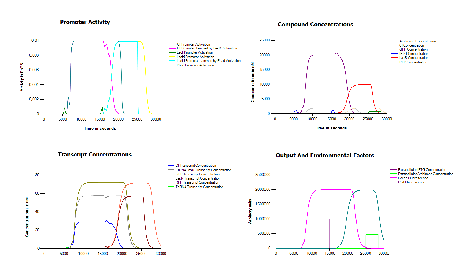
Because we did not manage to finish our complete device we decided to try and model our device in the Cumulus system without any measurement data. One of the main problems in assembling our device in the wetlab seemed to be the defective hybB promoter. For this reason we replaced it in this model with a LacI promoter. In order to operate our system we also assume that we can remove both arabinose and IPTG from the medium in an efficient way. As you can see, with these small modifications we get a perfectly working system.

This figure shows a simulation of our full model. As you can see in the bottom left corner we induce twice with IPTG for ten minutes, once after 5000 seconds and a second time after 15000 seconds, finally we reset the system with a long exposure to arabinose after 25000

Multiple experiments

It is also possible to use Cumulus to compare information from multiple experiments. Having partially different models. In this situation there is some additional accuracy gain from the better characterization of the overlapping BioBricks. Below we show an example with our characterization of the CI autoinducing-loops family. In this situation we have 12 contructs that all share two promoters but have different combinations of biobricks for degredation tags and ribosome binding sites.

This image shows the results of the simulation of the 12 autoinducing-loops from the CI family. Note that in three plots, the measurements, shown in other windows as green dots, are missing. These are the parts that had cloning errors (see wetlab result section).Even though we have no data on these constructs. We are still able however to get simulated results for these parts. This data is derived from how the BioBricks it uses preform in the other experiments