 "
"
Team:Grenoble/Projet/Modelling/Deterministic
From 2011.igem.org
BouGeo7314 (Talk | contribs) |
JeanBaptiste (Talk | contribs) |
||
| (15 intermediate revisions not shown) | |||
| Line 6: | Line 6: | ||
<html> | <html> | ||
| + | |||
| + | <!-- | ||
| + | <img src="http://www.clickartists.org/clicksite/html/images/square.jpg"/> | ||
| + | <h2>JB</h2> | ||
| + | |||
| + | |||
| + | <!-- | ||
| + | Si vous éditez la page commencez par décommenter ces lignes, publier, PUIS commencer à faire ce que vous avez à faire et quand vous avez fini de publier remettez en commentaire. | ||
| + | |||
| + | Ne laissez pas le carré trop longtemps si vous n'éditez pas, chaque fois reprenez ce qui est sur internet plutôt que ce que vous avez sur votre PC | ||
| + | ps: dans Geany selectionner une ou plusieurs lignes et appuyer sur "Ctrl + E" pour commenter ou décommenter | ||
| + | --> | ||
<div class="body"> | <div class="body"> | ||
| + | |||
| + | |||
| + | |||
| + | |||
| + | <center> | ||
| + | <form method="get" > | ||
| + | <input type="button" value="< PREVIOUS <" onclick="document.location = '/Team:Grenoble/Projet/Modelling';" /> | ||
| + | <select name="id" onchange="document.location = '/Team:Grenoble/Projet/Modelling' + this.options[this.selectedIndex].value ;"> | ||
| + | |||
| + | <optgroup label="Modelling Homepage"> | ||
| + | |||
| + | <option value="#Content" >Table of content</option> | ||
| + | |||
| + | </optgroup> | ||
| + | |||
| + | <optgroup label="Construction of the model" > | ||
| + | |||
| + | <option value="/Deterministic#Our_EquationsTS" selected="selected">Establishment of the equation - Toggle switch</option> | ||
| + | |||
| + | <option value="/Deterministic#Our_EquationsQS" >Establishment of the equation - Quorum sensing</option> | ||
| + | |||
| + | <option value="/Deterministic#Our_algorithms" >Our algorithms</option> | ||
| + | |||
| + | |||
| + | </optgroup> | ||
| + | |||
| + | <optgroup label="Stochastic Modelling"> | ||
| + | |||
| + | <option value="/Stochastic#Geof">Sensitivity to noise</option> | ||
| + | |||
| + | <option value="/Stochastic#Gillespie_algorithm">Gillespie algorithm</option> | ||
| + | |||
| + | <option value="/Stochastic#Stats">Mean, standard deviation and stats</option> | ||
| + | |||
| + | </optgroup> | ||
| + | |||
| + | <optgroup label="Parameters"> | ||
| + | |||
| + | <option value="/Parameters">Table of parameters</option> | ||
| + | |||
| + | </optgroup> | ||
| + | </select> | ||
| + | <input type="hidden" name="id2" value="0" /> | ||
| + | <input type="submit" value="Go!" /> | ||
| + | <input type="button" value="> NEXT >" onclick="document.location = '/Team:Grenoble/Projet/Modelling/Stochastic';" /> | ||
| + | |||
| + | </form> | ||
| + | </center> | ||
| + | |||
| + | |||
<div class="left"> | <div class="left"> | ||
| Line 13: | Line 75: | ||
<h1>Construction of the model</h1> | <h1>Construction of the model</h1> | ||
| - | <a href="http://2011. | + | <a href="http://2011..org/wiki/images/d/d1/Rapport_Equations.pdf"> |
<img src="http://2011.iGEM.org/wiki/skins/common/images/icons/fileicon-pdf.png" style="float: left; height: 20px; width: auto"> | <img src="http://2011.iGEM.org/wiki/skins/common/images/icons/fileicon-pdf.png" style="float: left; height: 20px; width: auto"> | ||
PDF version of the next two sections (Equations for Toggle Switch and Quorum sensing)</a><br/> | PDF version of the next two sections (Equations for Toggle Switch and Quorum sensing)</a><br/> | ||
| + | <!-- | ||
<div class="noindent"><p>You need MathML supported on your browser to read the equations on this page. However, | <div class="noindent"><p>You need MathML supported on your browser to read the equations on this page. However, | ||
you can find these equations in the above PDF version.</p> | you can find these equations in the above PDF version.</p> | ||
</div> | </div> | ||
| + | --> | ||
<p> As a proof of concept, we will consider anhydrotetracycline (aTc) instead of Mercury in | <p> As a proof of concept, we will consider anhydrotetracycline (aTc) instead of Mercury in | ||
| Line 34: | Line 98: | ||
</div> | </div> | ||
| - | <div class="blocbackground" id=" | + | <div class="blocbackground" id="Two_level"> |
| - | + | <h2>The Two modules of Modelling</h2> | |
| - | + | ||
<p> | <p> | ||
| - | + | Large-scale biochemical networks are classically decomposed into modules of smaller size to facilitate | |
| + | the model building process and the model calibration. The approach consists in modelling each module | ||
| + | separately and integrating the different models into a larger model of the whole system. | ||
| + | Like divided our genetic network in severals part (see <a href="https://2011.igem.org/Team:Grenoble/Projet/Design">genetic network</a>), | ||
| + | we also divided our model in two independant level of modelling: | ||
<ul> | <ul> | ||
| - | <li><strong>Toggle Switch | + | <li><strong>The Toggle Switch module:</strong> modelling this network module allows to predict in |
| - | <li><strong>Quorum Sensing and Coloration:</strong> | + | which state the bacteria are. In particular, we can determine the switching conditions in bacteria |
| + | and the localization of the switching area on the device (that depend on both IPTG and aTc | ||
| + | concentrations). This gives indications on how to adjust the size of the device to improve the | ||
| + | aTc detection.</li> | ||
| + | <li><strong>The Quorum Sensing and Coloration module:</strong>the corresponding model is used to | ||
| + | predict the localization and the width of the red line on the device. The modelling results are | ||
| + | used to improve the device precision, for instance, by choosing between a device with a continuous | ||
| + | bacterial layer and a device with strips containing bacteria. Each strip has the same concentration | ||
| + | of aTc, but a different IPTG concentration.</li> | ||
</ul> | </ul> | ||
</p> | </p> | ||
<p> | <p> | ||
The first level of the model will allow us to define the switch conditions in bacteria, depending | The first level of the model will allow us to define the switch conditions in bacteria, depending | ||
| - | on the concentrations of | + | on the concentrations of aTc and IPTG. From these results, we could see where the switch |
zone will appear on the device and therefore, the position of the red line. These parts of the | zone will appear on the device and therefore, the position of the red line. These parts of the | ||
| - | results indicate the range of | + | results indicate the range of aTc that can be detected. |
</p> | </p> | ||
<p> | <p> | ||
| - | The second level will | + | The second level will give us an estimation of the red line width, which indicates the system precision. |
| - | + | Based on these results, we could improve the precision of our device, for instance, by comparing | |
between a device with a continuous bacterial layer and a device with strips containing bacteria. | between a device with a continuous bacterial layer and a device with strips containing bacteria. | ||
Each strip has a different IPTG concentration, but the same concentration of Mercury. | Each strip has a different IPTG concentration, but the same concentration of Mercury. | ||
</p> | </p> | ||
| - | <p><strong>Two independent levels of modelling which are coupled in order to get a global simulation of | + | <p><strong>Two independent levels of modelling which are coupled in order to get a |
| - | + | <a href="https://2011.igem.org/Team:Grenoble/Projet/Results/Toggle#TS_QS">global simulation of the device.</a> | |
| - | + | </strong></p> | |
| + | </div> | ||
| + | <div class="blocbackground" id="Our_EquationsTS"> | ||
| + | <h2>Establishment of the equation</h2> | ||
<h3>Toggle switch</h3> | <h3>Toggle switch</h3> | ||
| - | <p>In a first part, we define a model to caracterize the Toggle Switch | + | <p>In a first part, we define a model to caracterize the <a href="https://2011.igem.org/Team:Grenoble/Projet/Design/toggle">Toggle Switch module</a> of our genetic network. |
| - | + | <br/></p> | |
| - | + | ||
| - | + | ||
<ol> | <ol> | ||
| - | <li>Biological | + | <li>Biological Model</li> |
<p> | <p> | ||
A toggle switch consists of two genes, each coding for a protein | A toggle switch consists of two genes, each coding for a protein | ||
| Line 78: | Line 154: | ||
<p> | <p> | ||
The biological system we are trying to implement is more complex, | The biological system we are trying to implement is more complex, | ||
| - | on both the biological and physical side. However, the toggle | + | on both the biological and physical side. However, the toggle switch |
| - | + | model is basically the same. In the study of the toggle switch itself, | |
| - | + | the system can be reduced to a simple two-state subsystem that we will | |
| - | subsystem that we will then use for the rest of our modelling. The | + | then use for the rest of our modelling. However, our toggle switch model |
| + | is basically the same: we can reduce it to a simple two-state subsystem | ||
| + | that we will then use for the rest of our modelling. The | ||
toggle switch itself is not influenced by the rest of the system, | toggle switch itself is not influenced by the rest of the system, | ||
if we do not consider the RsmA regulatory system that will be | if we do not consider the RsmA regulatory system that will be | ||
| Line 89: | Line 167: | ||
</p> | </p> | ||
| - | <li>Mathematical | + | <li>Mathematical Model</li> |
<p> | <p> | ||
| - | |||
In order to get the state of the bacteria, we need to compute the concentration of both | In order to get the state of the bacteria, we need to compute the concentration of both | ||
| - | repressors. To obtain these | + | repressors. To obtain these variations, we develop a system of ordinary differential equations (ODES) |
| - | the behavior of the Toggle Switch. | + | which governs the behavior of the Toggle Switch. |
</p> | </p> | ||
<center> | <center> | ||
| Line 100: | Line 177: | ||
\frac{d[TetR]}{dt} = \frac{k_{pLac}.[pLac]_{tot}}{1 + (\frac{[lacI]}{K_{pLac} + \frac{K_{pLac}.[IPTG]}{K_{lacI-IPTG}}.})^\beta} - \delta_{TetR}.[TetR]$ | \frac{d[TetR]}{dt} = \frac{k_{pLac}.[pLac]_{tot}}{1 + (\frac{[lacI]}{K_{pLac} + \frac{K_{pLac}.[IPTG]}{K_{lacI-IPTG}}.})^\beta} - \delta_{TetR}.[TetR]$ | ||
<br/><br/> | <br/><br/> | ||
| - | $\frac{d[lacI]}{dt} = \frac{k_{pTet}.[pTet]_{tot}}{1 + (\frac{[ | + | $\frac{d[lacI]}{dt} = \frac{k_{pTet}.[pTet]_{tot}}{1 + (\frac{[tetR]}{K_{pTet} + \frac{K_{pTet}.[aTc]}{K_{TetR-aTc}}.})^\gamma} - \delta_{lacI}.[lacI]$ |
</center> | </center> | ||
<p> | <p> | ||
| - | + | With this ODE system, we follow the evolution of the concentration of the two toggle switch repressors, | |
| - | + | TetR and LacI. This gives us the state of the bacteria. A demonstration of this ODE system is available | |
| - | + | in the previous pdf file. We briefly explain the equations below. | |
| - | + | ||
| - | + | ||
</p> | </p> | ||
<p> | <p> | ||
| - | Both equations are | + | Both equations are developed following the same approach. There is a term of production and a term of |
| - | + | degradation. The parameters $k_{pLac}.[pLac]_{tot}$ represent the protein synthesis rate from the pLac promoter. | |
| - | pLac | + | K_{pLac} and K_{lacI−IPTG} are the dissociation constants of LacI and pLac, and LacI and IPTG, respectively. |
| - | + | The parameters β and γ denote the cooperativity of repression, that is, the number of repressors bound | |
| - | + | to the promoter. | |
</p> | </p> | ||
<p> | <p> | ||
| - | + | According to these equations, the rate of variation of repressor TetR is inhibited by the repressor LacI. | |
| - | + | The degree of inhibition is modulated by the IPTG concentration. Reciprocally in the second equation, | |
| - | + | the rate of variation of LacI depends on TetR, whose negative effect is modulated by aTc. | |
| - | + | ||
</p> | </p> | ||
<p><strong> | <p><strong> | ||
| Line 132: | Line 206: | ||
</ol> | </ol> | ||
| + | <p> | ||
| + | With this model, we were able to predict the <a href="https://2011.igem.org/Team:Grenoble/Projet/Results/Toggle#TS_QS">behavior of our toggle switch</a>. | ||
| + | </p> | ||
</div> | </div> | ||
<div class="blocbackground" id="Our_EquationsQS"> | <div class="blocbackground" id="Our_EquationsQS"> | ||
| Line 137: | Line 214: | ||
<h3>Quorum sensing</h3> | <h3>Quorum sensing</h3> | ||
<ol> | <ol> | ||
| - | <li>Mathematical | + | <li>Mathematical Model</li> |
<p> | <p> | ||
| - | In a second part, we define a model able to | + | In a second part, we define a model able to characterize the <a href="https://2011.igem.org/Team:Grenoble/Projet/Design/quorum">quorum sensing module</a> of our genetic network, |
| - | + | which involves the quorum sensing genes CinI and CinR, as well as the signaling molecule AHL.<br/> | |
| - | + | ||
| - | + | In order to model the Quorum Sensing module, we detail below the different reactions taking place | |
| - | + | inside this module. For reasons that will become clear later, we focus on a particular area of our | |
| - | + | device, where neighboring bacteria will have a different behavior, although they carry the same | |
| - | + | genetic circuit. | |
| - | + | ||
| - | + | ||
| - | + | ||
| - | the | + | |
| - | + | ||
| - | + | ||
| - | + | ||
| - | + | ||
| - | + | ||
| - | + | ||
| - | + | ||
| - | + | ||
| - | + | ||
| - | + | ||
| - | + | ||
| - | + | ||
| - | + | ||
| - | + | ||
| - | + | ||
</p> | </p> | ||
<img src="https://static.igem.org/mediawiki/2011/a/a5/QS_details_2.png" class="centerwide" style="bow-shadow: non"/> | <img src="https://static.igem.org/mediawiki/2011/a/a5/QS_details_2.png" class="centerwide" style="bow-shadow: non"/> | ||
| - | <div class="legend"><strong>Figure 1:</strong> | + | <div class="legend"><strong>Figure 1:</strong>Mechanism of Quorum Sensing diffusion at the boundary</div> |
<p> | <p> | ||
| - | According to the figure, several | + | According to the figure, several must be taken into account: |
<ol> | <ol> | ||
<li>the production of the Quorum Sensing molecule</li> | <li>the production of the Quorum Sensing molecule</li> | ||
| Line 182: | Line 240: | ||
To model these mecanisms, we need to follow the evolution of the following quantities | To model these mecanisms, we need to follow the evolution of the following quantities | ||
<ul> | <ul> | ||
| - | <li>$[QS_i]$ concentration of the intracellular Quorum Sensing.</li> | + | <li>$[QS_i]$ concentration of the intracellular Quorum Sensing molecule.</li> |
| - | <li>$[QS_e]$ concentration of the extracellular Quorum Sensing.</li> | + | <li>$[QS_e]$ concentration of the extracellular Quorum Sensing molecule.</li> |
<li>$[cinR]$ concentration of the Quorum Sensing receptor.</li> | <li>$[cinR]$ concentration of the Quorum Sensing receptor.</li> | ||
<li>$[cinI]$ concentration of the Quorum Sensing producer enzyme.</li> | <li>$[cinI]$ concentration of the Quorum Sensing producer enzyme.</li> | ||
| Line 196: | Line 254: | ||
$\frac{d[QS_e]}{dt} = \rho v_c\eta([QS_i]-[QS_e])-\delta_{QSe} [QS_e] + D_{diff}\frac{\partial^2 [QS_e]}{\partial x^2}$<br/><br/> | $\frac{d[QS_e]}{dt} = \rho v_c\eta([QS_i]-[QS_e])-\delta_{QSe} [QS_e] + D_{diff}\frac{\partial^2 [QS_e]}{\partial x^2}$<br/><br/> | ||
$\frac{d[cinR_{free}]}{dt} = \frac{k_{pLac}.[pLac]_{tot}}{1 + (\frac{[lacI_{total}]}{K_{pLac} + \frac{K_{pLac}.[IPTG]}{K_{lacI-IPTG}}.})^\beta} - \delta_{cinR}[cinR_{free}] - V_{complexation}$<br/><br/> | $\frac{d[cinR_{free}]}{dt} = \frac{k_{pLac}.[pLac]_{tot}}{1 + (\frac{[lacI_{total}]}{K_{pLac} + \frac{K_{pLac}.[IPTG]}{K_{lacI-IPTG}}.})^\beta} - \delta_{cinR}[cinR_{free}] - V_{complexation}$<br/><br/> | ||
| - | $\frac{[cinR_{comp}]}{} = K_{comp}([cinR_{free}].[QS_i])$<br/><br/> | + | $\frac{d[cinR_{comp}]}{dt} = K_{comp}([cinR_{free}].[QS_i])$<br/><br/> |
</center> | </center> | ||
<p> | <p> | ||
| - | In the first equation, expressing the evolution of intracellular Quorum Sensing, 3 terms are involved: $[ | + | In the first equation, expressing the evolution of the concentration of the intracellular Quorum Sensing |
| - | $\delta_{QSi} [ | + | molecule, 3 terms are involved: $[QSe]−[QSi]$, which describes the diffusion through the membrane, |
| + | $\delta_{QSi}[QSi]$, the degradation and $k_{QS−production}[cinI]$, the production of Quorum Sensing molecule | ||
| + | by the enzyme CinI. | ||
In the second equation, expressing the evolution of extracellular Quorum Sensing, there is no production term, but a spatial diffusion term | In the second equation, expressing the evolution of extracellular Quorum Sensing, there is no production term, but a spatial diffusion term | ||
$D_{diff}\frac{\partial^2 [QS_e]}{\partial x^2}$. | $D_{diff}\frac{\partial^2 [QS_e]}{\partial x^2}$. | ||
</p> | </p> | ||
<p> | <p> | ||
| - | + | The concentrations of CinI and CinR can be obtained by using the toggle switch modelling. Indeed, since CinI | |
| - | + | is on the pathway of LacI and CinR on the pathway of Tet, their evolution follow the same equations. | |
| - | the complexation of | + | In addition we consider the complexation of the CinR protein and the Quorum Sensing molecule, |
| - | + | which is expressed by the term $V_{complexation}$ in the CinR equation: | |
| - | + | \[V_{complexation} = K_{comp}[QS_i][CinR_{free}]\] | |
| + | with $K_{comp}$ the affinity constant of AHL for cinR. | ||
</p> | </p> | ||
<p> | <p> | ||
| - | In order to simplify the model, we considered that the complexation is | + | In order to simplify the model, we considered that the complexation of CinR to AHL is total and depends only |
| - | + | on $[cinR]$ and $[QS_i] which is the limitant factor$. | |
</p> | </p> | ||
<p><strong> | <p><strong> | ||
| - | To solve this set of | + | To solve this set of equations, we couldn't use a classical ODE solver from Matlab (Mathworks), because |
| - | + | the equations are derived both in time and space. We therefore needed to use the finite difference method. | |
| - | + | To that aim, we build a matrix based on Taylor's series discretization. | |
</strong></p> | </strong></p> | ||
| Line 231: | Line 292: | ||
$M_{QSe}(m+1,n+1) = [QS_e](x + dx,t+dt)$ | $M_{QSe}(m+1,n+1) = [QS_e](x + dx,t+dt)$ | ||
</center> | </center> | ||
| + | <p> | ||
| + | In these equations, m represents the spatial dimension and n the temporal dimension. | ||
| + | </p> | ||
<img src="http://2011.iGEM.org/wiki/images/c/c6/Matrix_QS.png" class="centerwide" style="box-shadow: none"/> | <img src="http://2011.iGEM.org/wiki/images/c/c6/Matrix_QS.png" class="centerwide" style="box-shadow: none"/> | ||
<ul> | <ul> | ||
| Line 249: | Line 313: | ||
</li> | </li> | ||
<li> | <li> | ||
| - | Of course, | + | Of course, QSi, CinI and CinR matrices will be similarly implemented. |
</li> | </li> | ||
</ul> | </ul> | ||
| Line 255: | Line 319: | ||
<li>Discretization of the equation</li> | <li>Discretization of the equation</li> | ||
<p> | <p> | ||
| - | With our continuous equations set, we want to obtain discrete definition of each of the matrices. | + | With our continuous equations set, we want to obtain discrete definition of each of the matrices. interdependencies |
| - | + | of the equations imply that the computation of the matrices will be performed on the entire CinI matrix | |
| - | first, then each line of the Qi and Qe matrices will be computed alternatively. | + | first, then each line of the Qi and Qe matrices will be computed alternatively. The computation of the CinR |
| - | will be performed. | + | will be eventually performed. |
</p> | </p> | ||
<p> | <p> | ||
| Line 274: | Line 338: | ||
$<br/><br/> | $<br/><br/> | ||
$ | $ | ||
| - | + | with D_{m} =\rho v_c \eta .M_{QSi}(m,n) - M_{QSe}(m,n)(\delta_{QSe} + \rho v_c \eta) | |
$<br/><br/> | $<br/><br/> | ||
$ | $ | ||
| - | M_{CinR_{free}}(m,n+1) = \Delta t (\frac{k_{pTet}[P_{ | + | M_{CinR_{free}}(m,n+1) = \Delta t (\frac{k_{pTet}[P_{Tet total}]}{1+ (\frac{[TetR]}{K_{pTet}(1+\frac{[aTc]}{K_{TetR - aTc}})})^{n_{pTet}}} - M_{CinR_{free}}(m,n)(\delta_{CinR} - k_{comp}.M_{Qi}(m,n))) + M_{CinR_{free}}(m,n)$<br/> |
</center> | </center> | ||
| - | <p> | + | <p><strong> |
With these discrete equations the 4 matrices can be computed through simple calculation loops over each line. | With these discrete equations the 4 matrices can be computed through simple calculation loops over each line. | ||
The CinI matrix does not depend on space dimension, it is then possible to compute it without discretization with | The CinI matrix does not depend on space dimension, it is then possible to compute it without discretization with | ||
| - | a differential solver. | + | a differential solver.</strong> |
| + | </p> | ||
| + | |||
| + | <p><strong> | ||
| + | Moreover to get the coupling of toggle switch and quorum sensing modules, we used the results of the first one | ||
| + | (lacI and TetR evolution) to get the evolution of quorum sensing proteins (respectively cinI and cinR). | ||
| + | It means that the output of the first module are used as input for the second module.</strong> | ||
| + | </p> | ||
| + | |||
| + | <p> | ||
| + | With this model, we were able to predict how the <a href="https://2011.igem.org/Team:Grenoble/Projet/Results/Toggle#QS">red stripe appears</a> on the plate | ||
</p> | </p> | ||
| Line 293: | Line 367: | ||
<h2>Our algorithms</h2> | <h2>Our algorithms</h2> | ||
<p> | <p> | ||
| - | + | An archive containing our Matlab scripts for the deterministic modeling can be found <a href="http://iGEMgrenoble-files.perso.sfr.fr/2011/MATLAB_Archives/">here</a> | |
| - | + | (file Deterministic_archive.tar.gz). You can launch and ODE-based simulation(see our ODEs in | |
| - | + | the two previous sections) with the file biosenseur1Dmain.m. | |
</p> | </p> | ||
<p> | <p> | ||
| - | Several dialog boxes will pop up to enter the specificities of the simulation : (physical | + | Several dialog boxes will pop up to enter the specificities of the simulation: (physical |
| - | specificities of the device, chemical species concentrations and IPTG gradient ) | + | specificities of the device, chemical species concentrations and IPTG gradient). |
</p> | </p> | ||
<p> | <p> | ||
| - | + | At the end of the simulation you obtain 3 matrices named M_stock, M_QS and M_comp containing the concentrations | |
| - | + | in each protein species at each time point and on each physical point of the plate. We wrote three Matlab scripts | |
| - | + | (DynamicplottingTS, DynamicplottingQS and DynamicplottingCP) that dynamically display the protein concentrations. | |
| - | + | For a good understanding of the models and of our results, we also wrote a script (Imageshow.m) to illustrate | |
| - | + | the plate coloration. | |
| + | </p> | ||
| + | |||
| + | <p> | ||
| + | To see the results we obtained with this algorithms, refer to this <a href="https://2011.igem.org/Team:Grenoble/Projet/Results">page</a>. | ||
| + | </p> | ||
</div> | </div> | ||
| - | < | + | <center> |
<form method="get" > | <form method="get" > | ||
| - | <input type="button" value="< PREVIOUS <" onclick="document.location = '/Team:Grenoble/Projet/Modelling | + | <input type="button" value="< PREVIOUS <" onclick="document.location = '/Team:Grenoble/Projet/Modelling';" /> |
<select name="id" onchange="document.location = '/Team:Grenoble/Projet/Modelling' + this.options[this.selectedIndex].value ;"> | <select name="id" onchange="document.location = '/Team:Grenoble/Projet/Modelling' + this.options[this.selectedIndex].value ;"> | ||
| Line 321: | Line 400: | ||
</optgroup> | </optgroup> | ||
| - | <optgroup label=" | + | <optgroup label="Construction of the model" > |
| - | <option value="/Deterministic#Our_EquationsTS" selected="selected"> | + | <option value="/Deterministic#Our_EquationsTS" selected="selected">Establishment of the equation - Toggle switch</option> |
| - | <option value="/Deterministic#Our_EquationsQS" > | + | <option value="/Deterministic#Our_EquationsQS" >Establishment of the equation - Quorum sensing</option> |
<option value="/Deterministic#Our_algorithms" >Our algorithms</option> | <option value="/Deterministic#Our_algorithms" >Our algorithms</option> | ||
| - | |||
| - | |||
| Line 336: | Line 413: | ||
<optgroup label="Stochastic Modelling"> | <optgroup label="Stochastic Modelling"> | ||
| - | <option value="/Stochastic#Geof"> | + | <option value="/Stochastic#Geof">Sensitivity to noise</option> |
<option value="/Stochastic#Gillespie_algorithm">Gillespie algorithm</option> | <option value="/Stochastic#Gillespie_algorithm">Gillespie algorithm</option> | ||
| Line 346: | Line 423: | ||
<optgroup label="Parameters"> | <optgroup label="Parameters"> | ||
| - | <option value="/Parameters"> | + | <option value="/Parameters">Table of parameters</option> |
| - | + | ||
| - | + | ||
| - | + | ||
| - | + | ||
| - | + | ||
| - | + | ||
| - | + | ||
| - | + | ||
</optgroup> | </optgroup> | ||
| Line 363: | Line 432: | ||
</form> | </form> | ||
| + | </center> | ||
| + | |||
</div> | </div> | ||
Latest revision as of 03:07, 29 October 2011
Construction of the model
As a proof of concept, we will consider anhydrotetracycline (aTc) instead of Mercury in our model, and the transcriptional regulator TetR in place of MerR. The TetR system is well characterized in E. coli, which facilitates the modelling. In addition, if the system works well with aTc, it should work as well with Mercury, Copper or lead for example.
In addition, since aTc diffuse freely accross the membrane of the cell, we do not have to take
complex uptake mechanisms into considerations. Mercury is ionized and its entry in the cells
depends on the presence of transporter protein.
So in the following chapter, we are going to use TetR instead of MerR and aTc instead of
Mercury.
The Two modules of Modelling
Large-scale biochemical networks are classically decomposed into modules of smaller size to facilitate the model building process and the model calibration. The approach consists in modelling each module separately and integrating the different models into a larger model of the whole system. Like divided our genetic network in severals part (see genetic network), we also divided our model in two independant level of modelling:
- The Toggle Switch module: modelling this network module allows to predict in which state the bacteria are. In particular, we can determine the switching conditions in bacteria and the localization of the switching area on the device (that depend on both IPTG and aTc concentrations). This gives indications on how to adjust the size of the device to improve the aTc detection.
- The Quorum Sensing and Coloration module:the corresponding model is used to predict the localization and the width of the red line on the device. The modelling results are used to improve the device precision, for instance, by choosing between a device with a continuous bacterial layer and a device with strips containing bacteria. Each strip has the same concentration of aTc, but a different IPTG concentration.
The first level of the model will allow us to define the switch conditions in bacteria, depending on the concentrations of aTc and IPTG. From these results, we could see where the switch zone will appear on the device and therefore, the position of the red line. These parts of the results indicate the range of aTc that can be detected.
The second level will give us an estimation of the red line width, which indicates the system precision. Based on these results, we could improve the precision of our device, for instance, by comparing between a device with a continuous bacterial layer and a device with strips containing bacteria. Each strip has a different IPTG concentration, but the same concentration of Mercury.
Two independent levels of modelling which are coupled in order to get a global simulation of the device.
Establishment of the equation
Toggle switch
In a first part, we define a model to caracterize the Toggle Switch module of our genetic network.
- Biological Model
- Mathematical Model
A toggle switch consists of two genes, each coding for a protein that represses the expression of the other gene. This double repression system ensures the basic function of a toggle switch: a bistable system which can be switched from one state to the other by putting, in our example, some IPTG or aTc molecules in the medium.
The biological system we are trying to implement is more complex, on both the biological and physical side. However, the toggle switch model is basically the same. In the study of the toggle switch itself, the system can be reduced to a simple two-state subsystem that we will then use for the rest of our modelling. However, our toggle switch model is basically the same: we can reduce it to a simple two-state subsystem that we will then use for the rest of our modelling. The toggle switch itself is not influenced by the rest of the system, if we do not consider the RsmA regulatory system that will be modeled at the very end of our work. Thus we will be able to model the toggle switch independently and then build the rest of the model upon this basis.
In order to get the state of the bacteria, we need to compute the concentration of both repressors. To obtain these variations, we develop a system of ordinary differential equations (ODES) which governs the behavior of the Toggle Switch.
$\frac{d[lacI]}{dt} = \frac{k_{pTet}.[pTet]_{tot}}{1 + (\frac{[tetR]}{K_{pTet} + \frac{K_{pTet}.[aTc]}{K_{TetR-aTc}}.})^\gamma} - \delta_{lacI}.[lacI]$
With this ODE system, we follow the evolution of the concentration of the two toggle switch repressors, TetR and LacI. This gives us the state of the bacteria. A demonstration of this ODE system is available in the previous pdf file. We briefly explain the equations below.
Both equations are developed following the same approach. There is a term of production and a term of degradation. The parameters $k_{pLac}.[pLac]_{tot}$ represent the protein synthesis rate from the pLac promoter. K_{pLac} and K_{lacI−IPTG} are the dissociation constants of LacI and pLac, and LacI and IPTG, respectively. The parameters β and γ denote the cooperativity of repression, that is, the number of repressors bound to the promoter.
According to these equations, the rate of variation of repressor TetR is inhibited by the repressor LacI. The degree of inhibition is modulated by the IPTG concentration. Reciprocally in the second equation, the rate of variation of LacI depends on TetR, whose negative effect is modulated by aTc.
This indicates that the two equations are coupled. And also that only one repressor could be predominant, as shown later.
These two equations can be easily computed with a differential solver. We can precisely estimate the effects of each parameter.
With this model, we were able to predict the behavior of our toggle switch.
Establishment of the equation
Quorum sensing
- Mathematical Model
- the production of the Quorum Sensing molecule
- the secretion of the molecule
- the diffusion of the molecule in the medium
- the penetration of the molecule
- the complexation of the molecule with its receptor
- the activation of the coloration
- $[QS_i]$ concentration of the intracellular Quorum Sensing molecule.
- $[QS_e]$ concentration of the extracellular Quorum Sensing molecule.
- $[cinR]$ concentration of the Quorum Sensing receptor.
- $[cinI]$ concentration of the Quorum Sensing producer enzyme.
- $[cinR_{comp}]$ concentration of the complexe cinR-QS.
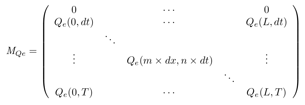
- Definition of the matrix
- On the spatial point of view, we only consider the x dimension, as the IPTG gradient will be only evolving along this dimension. Thus we consider the state of our cells is the same along the width of our plate.
- With this Matrix, and after computation of all the terms, we can get the entire behaviour of CinI, CinR, QS inside and outside the cells.
- The first line of the Matrix equals 0. These are the initial conditions we set to 0 at time t = 0s.
- On the borders of the plate (x = 0 and x = L) the model used has to be different, limit conditions will be set.
- Of course, QSi, CinI and CinR matrices will be similarly implemented.
- Discretization of the equation
In a second part, we define a model able to characterize the quorum sensing module of our genetic network,
which involves the quorum sensing genes CinI and CinR, as well as the signaling molecule AHL.
In order to model the Quorum Sensing module, we detail below the different reactions taking place
inside this module. For reasons that will become clear later, we focus on a particular area of our
device, where neighboring bacteria will have a different behavior, although they carry the same
genetic circuit.

According to the figure, several must be taken into account:
To model these mecanisms, we need to follow the evolution of the following quantities
Based on the Bangalore 2007 iGEM team, we get the following system of equations:
$\frac{d[QS_e]}{dt} = \rho v_c\eta([QS_i]-[QS_e])-\delta_{QSe} [QS_e] + D_{diff}\frac{\partial^2 [QS_e]}{\partial x^2}$
$\frac{d[cinR_{free}]}{dt} = \frac{k_{pLac}.[pLac]_{tot}}{1 + (\frac{[lacI_{total}]}{K_{pLac} + \frac{K_{pLac}.[IPTG]}{K_{lacI-IPTG}}.})^\beta} - \delta_{cinR}[cinR_{free}] - V_{complexation}$
$\frac{d[cinR_{comp}]}{dt} = K_{comp}([cinR_{free}].[QS_i])$
In the first equation, expressing the evolution of the concentration of the intracellular Quorum Sensing molecule, 3 terms are involved: $[QSe]−[QSi]$, which describes the diffusion through the membrane, $\delta_{QSi}[QSi]$, the degradation and $k_{QS−production}[cinI]$, the production of Quorum Sensing molecule by the enzyme CinI. In the second equation, expressing the evolution of extracellular Quorum Sensing, there is no production term, but a spatial diffusion term $D_{diff}\frac{\partial^2 [QS_e]}{\partial x^2}$.
The concentrations of CinI and CinR can be obtained by using the toggle switch modelling. Indeed, since CinI is on the pathway of LacI and CinR on the pathway of Tet, their evolution follow the same equations. In addition we consider the complexation of the CinR protein and the Quorum Sensing molecule, which is expressed by the term $V_{complexation}$ in the CinR equation: \[V_{complexation} = K_{comp}[QS_i][CinR_{free}]\] with $K_{comp}$ the affinity constant of AHL for cinR.
In order to simplify the model, we considered that the complexation of CinR to AHL is total and depends only on $[cinR]$ and $[QS_i] which is the limitant factor$.
To solve this set of equations, we couldn't use a classical ODE solver from Matlab (Mathworks), because the equations are derived both in time and space. We therefore needed to use the finite difference method. To that aim, we build a matrix based on Taylor's series discretization.
To solve this set of equations we have to use a matrix that will describe our system in both space and time. for example for the QS molecule outside of the cell :
$M_{QSe}(m+1,n+1) = [QS_e](x + dx,t+dt)$
In these equations, m represents the spatial dimension and n the temporal dimension.
With our continuous equations set, we want to obtain discrete definition of each of the matrices. interdependencies of the equations imply that the computation of the matrices will be performed on the entire CinI matrix first, then each line of the Qi and Qe matrices will be computed alternatively. The computation of the CinR will be eventually performed.
Parallel computation of all the matrices without proper control is not possible indeed, as the terms of Qi matrix will depend on the Qe terms of the preceding line (and vice-versa). Discretization is obtained with first order taylor series :
$ M_{QSe}(m,n+1) =\Delta t ( D_{m} + D_{diff} \frac{M_{QSe}(m+1,n) - 2 M_{QSe}(m,n) + M_{QSe}(m-1,n)}{\Delta x^2}) + M_{QSe}(m,n) $
$ with D_{m} =\rho v_c \eta .M_{QSi}(m,n) - M_{QSe}(m,n)(\delta_{QSe} + \rho v_c \eta) $
$ M_{CinR_{free}}(m,n+1) = \Delta t (\frac{k_{pTet}[P_{Tet total}]}{1+ (\frac{[TetR]}{K_{pTet}(1+\frac{[aTc]}{K_{TetR - aTc}})})^{n_{pTet}}} - M_{CinR_{free}}(m,n)(\delta_{CinR} - k_{comp}.M_{Qi}(m,n))) + M_{CinR_{free}}(m,n)$
With these discrete equations the 4 matrices can be computed through simple calculation loops over each line. The CinI matrix does not depend on space dimension, it is then possible to compute it without discretization with a differential solver.
Moreover to get the coupling of toggle switch and quorum sensing modules, we used the results of the first one (lacI and TetR evolution) to get the evolution of quorum sensing proteins (respectively cinI and cinR). It means that the output of the first module are used as input for the second module.
With this model, we were able to predict how the red stripe appears on the plate
Our algorithms
An archive containing our Matlab scripts for the deterministic modeling can be found here (file Deterministic_archive.tar.gz). You can launch and ODE-based simulation(see our ODEs in the two previous sections) with the file biosenseur1Dmain.m.
Several dialog boxes will pop up to enter the specificities of the simulation: (physical specificities of the device, chemical species concentrations and IPTG gradient).
At the end of the simulation you obtain 3 matrices named M_stock, M_QS and M_comp containing the concentrations in each protein species at each time point and on each physical point of the plate. We wrote three Matlab scripts (DynamicplottingTS, DynamicplottingQS and DynamicplottingCP) that dynamically display the protein concentrations. For a good understanding of the models and of our results, we also wrote a script (Imageshow.m) to illustrate the plate coloration.
To see the results we obtained with this algorithms, refer to this page.