Team:Wageningen UR/Project/ModelingProj1
From 2011.igem.org
(→Modeling synchronized oscillations) |
(→Modeling synchronized oscillations) |
||
| Line 28: | Line 28: | ||
{{:Team:Wageningen_UR/Templates/Style | text= __NOTOC__ | {{:Team:Wageningen_UR/Templates/Style | text= __NOTOC__ | ||
| + | <!-- | ||
=== Short repetition of the Hasty construct used as base for our system === | === Short repetition of the Hasty construct used as base for our system === | ||
| Line 43: | Line 44: | ||
[[Team:Wageningen_UR/Project/ModelingProj1#Modeling_synchronized_oscillations| back to top]] | [[Team:Wageningen_UR/Project/ModelingProj1#Modeling_synchronized_oscillations| back to top]] | ||
| + | --> | ||
=== Mathematical model of the Hasty construct === | === Mathematical model of the Hasty construct === | ||
| - | Since our bio bricked oscillatory system is based on the | + | Since our bio bricked oscillatory system is based on the circuit published by Danino et al. in the paper [http://www.nature.com/nature/journal/v463/n7279/abs/nature08753.html “A synchronized quorum of genetic clocks”], in our team commonly referred to as the "Hasty construct", our first model of the system is a reproduction of the mathematical model in the [http://www.nature.com/nature/journal/v463/n7279/suppinfo/nature08753.html supplementary information] accompanying the publication mentioned. In their simulations, Danino et al. used a set of delay differential equations, which we also used as starting point for our modeling work. |
| - | + | <!-- | |
[[File:Equations_hasty_WUR.png|350px|left]] | [[File:Equations_hasty_WUR.png|350px|left]] | ||
| Line 63: | Line 65: | ||
|} | |} | ||
| - | {{:Team:Wageningen_UR/Templates/Style | text= __NOTOC__ | + | {{:Team:Wageningen_UR/Templates/Style | text= __NOTOC__ --> |
| + | The steps (transcription, translation, maturation etc.) from the luxI and aiiA genes to the corresponding proteins are not modeled separately, but the delay of the correlation between the internal AHL concentration, which triggers the expression of the genes, and the corresponding AiiA and LuxI is simulated by a Hill function which takes the history of the system into account, i.e. the concentration of AHL at the time it binds to LuxR to form the activation complex. | ||
| - | + | <!-- [[File:Equations2_hasty_WUR.png|150px]] | |
| - | + | ||
| - | + | ||
| - | + | ||
| - | [[File:Equations2_hasty_WUR.png|150px]] | + | |
| Line 78: | Line 77: | ||
in which tau represents the time step. It can be seen that the function takes the history of the system into account, since the production of the proteins depend on the past concentration of internal AHL as in: [[File:Equations3_hasty_WUR.png]]. | in which tau represents the time step. It can be seen that the function takes the history of the system into account, since the production of the proteins depend on the past concentration of internal AHL as in: [[File:Equations3_hasty_WUR.png]]. | ||
| - | + | --> | |
[[Team:Wageningen_UR/Project/ModelingProj1#Modeling_synchronized_oscillations| back to top]] | [[Team:Wageningen_UR/Project/ModelingProj1#Modeling_synchronized_oscillations| back to top]] | ||
| Line 84: | Line 83: | ||
=== Writing a modeling tool in matlab === | === Writing a modeling tool in matlab === | ||
| - | + | <!-- | |
[[File:Oscillation_GUI_WUR.png|center]] | [[File:Oscillation_GUI_WUR.png|center]] | ||
| - | '''Fig.2:''' ''GUI of the matlab modeling tool created by team Wageningen UR'' | + | '''Fig.2:''' ''GUI of the matlab modeling tool created by team Wageningen UR'' --> |
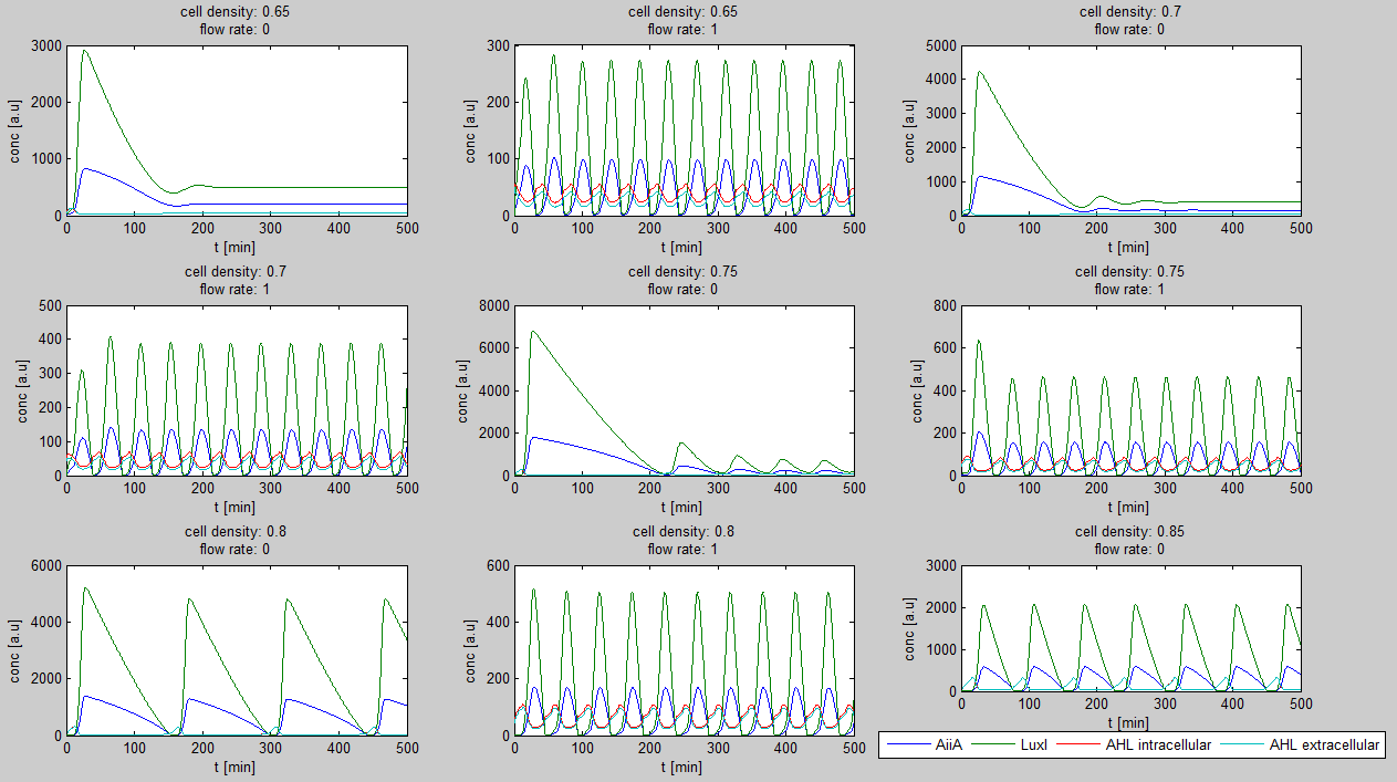
| - | For the first simulations, the same values for the parameters were used as in the cited paper and can be found in the [http://www.nature.com/nature/journal/v463/n7279/suppinfo/nature08753.html supplementary information]. To get graphs representing optimal oscillations, our team created a script for a matlab modeling tool which uses nested for-loops to vary the flow rate and cell density over a range of values. The resulting tool allows the user to enter the range in which the variables should be varied. The tool then iterates over the values and plots graphs of all combinations possible for that range of values. Figure 2 shows an example output of the tool. | + | For the first simulations, the same values for the parameters were used as in the cited paper and can be found in the [http://www.nature.com/nature/journal/v463/n7279/suppinfo/nature08753.html supplementary information]. To get graphs representing optimal oscillations, our team created a script for a matlab modeling tool which uses nested for-loops to vary the flow rate and cell density over a range of values. The resulting tool allows the user to enter the range in which the variables should be varied. The tool then iterates over the values and plots graphs of all combinations possible for that range of values. <!-- Figure 2 shows an example output of the tool. |
[[File:Example_output_graphs_WUR.png|770px|center]] | [[File:Example_output_graphs_WUR.png|770px|center]] | ||
| - | '''Fig.2:''' ''Variation of output graphs depending on the different starting conditions'' | + | '''Fig.2:''' ''Variation of output graphs depending on the different starting conditions'' --> |
Revision as of 19:14, 19 September 2011
 "
"


