Team:DTU-Denmark/Modeling
From 2011.igem.org
Modeling
Contents |
Motivation
A model is developed with the dual purpose of both developing hypotheses about the trap-RNA system and providing synthetic biologists the framework to characterize and incorporate the system into models of their designs. Several models for one-level sRNA-mRNA regulation exits in the literature[1][2], but the two-level regulation has not previously been quantitatively characterised nor modelled.
General kinetic model
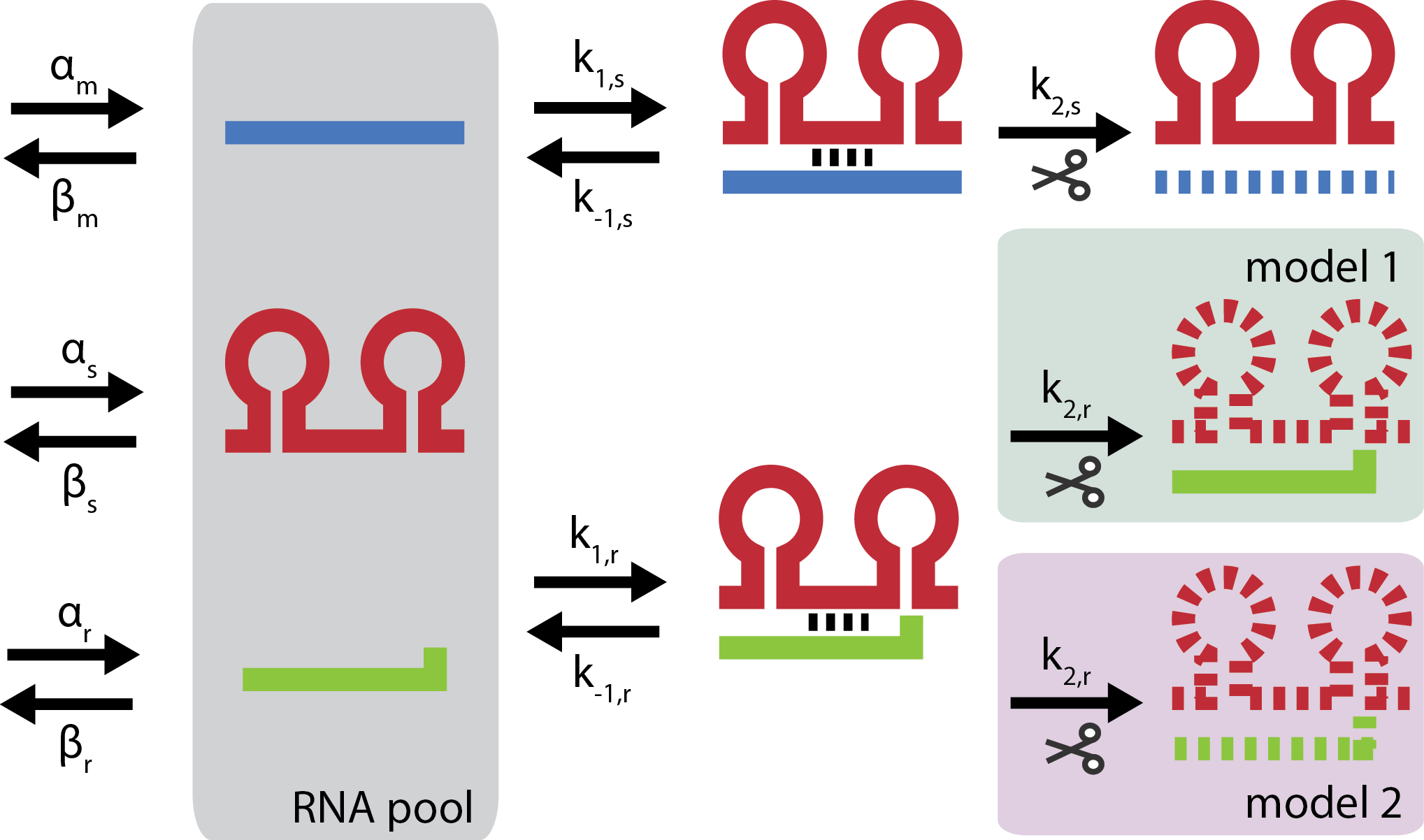
The modeling of the trap-RNA system is based on two general reaction schemes \begin{align} \color{blue} m + \color{red}s &\mathop{\rightleftharpoons}_{k_{-1,s}}^{k_{1,s}} c_{ms} \mathop{\rightarrow}^{k_{2,s}} (1 - p_s) \color{red} s \\ \color{red} s + \color{green} r &\mathop{\rightleftharpoons}_{k_{-1,r}}^{k_{1,r}} c_{sr} \mathop{\rightarrow}^{k_{2,r}} (1-p_r) \color{green} r \end{align}
In the first reaction ${\color{blue} m}$RNA binds to a ${\color{red}s}$RNA forming a complex called $c_{ms}$. The RNAs of the duplex are then irreversibly degraded with stoichiometries defined by $p_s$, which denotes the probability that $s$ is co-degraded in the reaction. The majority of investigated small regulatory RNA (srRNA) acts stoichiometrically, they are degraded 1:1 with their target mRNA corresponding to $p_s = 1$. Interestingly, studies indicate that the trap-RNA system acts catalytically with $p_s = 0$[3]. In the second reaction t$\color{green} r$ap-RNA inhibits the activity of the sRNA but the mechanism is unknown. The general scheme allows two different hypotheses; trap-RNA mediates degradation of the sRNA either catalytically or stoichiometrically.
In vivo genes and their RNAs are constantly being expressed and degraded giving rise to finite lifetimes of RNA molecules. To model the trap-RNA system in context of living cells the expression of each RNA is described by a production term $\alpha_i$ and the turnover of each RNA is described by a degradation term of first order $\beta_i[RNA]_i$.
\begin{equation} \label{proddeg} \mathop{\longrightarrow}^{production} [RNA]_i \mathop{\longrightarrow}^{degradation} \end{equation}
Eventually, the amount of RNA will settle into a steady-state where production equals degradation.
Ordinary differential equations (ODEs) are set up by applying the law of mass action to the general reaction scheme, the production and background degradation. The ODEs are then simplified by assuming pseudo-steady state of the RNA complexes $c_{ms} $ and $ c_{sr}$. In the general reaction scheme it follows (See ODEs) that
\begin{eqnarray} \label{system1} \frac{dm}{dt} &=& \alpha_m - \beta_m m - k_s ms \\ \label{system2} \frac{ds}{dt} &=& \alpha_s - \beta_s s - p_s k_s ms - k_r sr \\ \label{system3} \frac{dr}{dt} &=& \alpha_r - \beta_r r - p_r k_r sr \end{eqnarray}
where the kinetic constants of the general reaction scheme have been lumped into the overall kinetic constants $k_s = \frac{k_{1,s} k_{2,s}}{k_{-1,s} + k_{2,s}}$ and $k_r = \frac{k_{1,r} k_{2,r}}{k_{-1,r} + k_{2,r}}$. It is seen from the equations that setting either $p_s = 0$ or $p_r = 0$ simplifies the expression. Because $p_s = 0$ for the trap-RNA system whereas the value of $p_r$ is unknown, the general model is split up into two models; a catalytic and a partly stoichiometric trap-RNA mechanism corresponding to $p_r = 0$ or $0 < p_r \leq 1$ respectively.
Model 1: Catalytic trap-RNA
Assuming $p_s = 0$ and $p_r = 0$ the steady-state solution is derivable and unique. It is furthermore stable because all the eigen values of the Jacobian have negative real parts (see Steady-state). The steady-state of m is
\begin{equation} \label{ss} m^* = \frac{\alpha_m (\beta_r \beta_s + \alpha_r k_r)}{\beta_r \alpha_s k_s + \beta_m \beta_r \beta_s + \beta_m \alpha_r k_r} \end{equation}
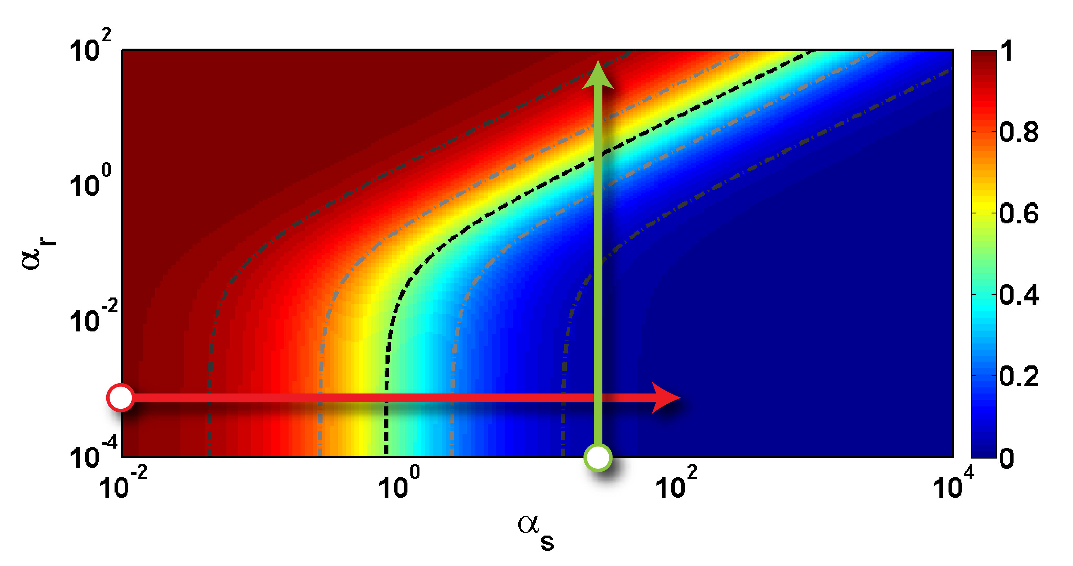
To eliminate the dependence on $\alpha_m$ the steady-state is scaled with respect to the maximum amount of expression $m^*_{max} = \frac{\alpha_m}{\beta_m}$. This maximum value of $m$ expression is achieved by not having any sRNA which is equivalent to $\alpha_s = 0$. A new measure of steady-state $\frac{m^*_{max}}{m^*}$ is interpreted as the fold repression caused by the system. To analyze how this fold repression depends on the variables and parameters, the steady-state solution is scaled and re-stated into its simpler form
\begin{equation} \label{phi1} \phi = \frac{m^*_{max}}{m^*} = 1 + \frac{\frac{k_s \alpha_s}{\beta_m \beta_s}}{1 + \frac{k_r \alpha_r}{\beta_s \beta_r}} \end{equation}
where $\phi$ is a measure of the fold repression.

Model 2: Partly stoichiometric trap-RNA
Assuming $p_s = 0$ and $0 < p_r \leq 1$ the steady-state solution with respect to m is \begin{equation} m^* = \frac{2}{\beta_m} \bigg( \frac{p_r \alpha_m \lambda_s}{\alpha_s p_r - \alpha_r -\lambda_r + 2 p_r \lambda_s + \sqrt{(\alpha_s p_r - \alpha_r - \lambda_r)^2 + 4 p_r \alpha_s \lambda_r}} \bigg) \end{equation} where $\lambda_r = \frac{\beta_s \beta_r}{k_r}$ and $\lambda_s = \frac{\beta_s \beta_m}{k_s}$. The fold repression is again defined removing the dependence on $\alpha_m$ \begin{equation} \label{phi2} \phi = \frac{m^*_{max}}{m^*} = 1 + \frac{\alpha_s p_r - \alpha_r -\lambda_r + \sqrt{(\alpha_s p_r - \alpha_r - \lambda_r)^2 + 4 p_r \alpha_s \lambda_r}}{2 p_r \lambda_s} \end{equation} The fold repression for the two models are reassuringly equivalent when $\alpha_r = 0$, which corresponds to ignoring the second reaction. This makes sense since the first reaction is identical for both dual degradation models.
| Parameter | Meaning | Unit |
|---|---|---|
| $\alpha_m$ | Transcription rate of target mRNA | [amount/time] |
| $\alpha_s$ | Transcription rate of sRNA (s) | [amount/time] |
| $\alpha_r$ | Transcription rate of sRNA (r) | [amount/time] |
| $\beta_m$ | Degradation rate of free mRNA | [1/time] |
| $\beta_s$ | Degradation rate of free sRNA (s) | [1/time] |
| $\beta_r$ | Degradation rate of free sRNA (r) | [1/time] |
| $p_s$ | Probability that s is codegraded with m | [-] |
| $p_r$ | Probability that r is codegraded with s | [-] |
| $k_s$ | Kinetic constant of sRNA mediated degradation of mRNA | [1/(time*amount)] |
| $k_r$ | Kinetic constant of trap-RNA mediated degradation of sRNA | [1/(time*amount)] |
| $\lambda_s$ | Leakage rate of sRNA mediated degradation of mRNA | [amount/time] |
| $\lambda_r$ | Leakage rate of trap-RNA mediated degradation of sRNA | [amount/time] |
Design of dynamic range

When only sRNA and target mRNA is present the steady-state of both model 1 and 2 is
\begin{equation} \label{lin} \phi = 1 + \frac{ \alpha_s}{\lambda_s} \end{equation}
which describes the baseline dynamic range corresponding to a dynamic range when changing the induction of sRNA, $\alpha_s$. Visually the baseline dynamic range corresponds to starting at the lower left corner of a heatmap and proceeding to the right.
The effect of the parameter $\lambda_s = \frac{\beta_m \beta_s}{k_s}$ on the baseline dynamic range is valid for both models and determines the sensitivity to $\alpha_s$.
Taking trap-RNA into account adds another component to the dynamic range. For model 1, the dynamic range of the fold repression when changing the induction of trap-RNA, $\alpha_r$, is described by the function
\begin{equation} \phi(\alpha_r) = 1 + \frac{\lambda_s^{-1} \alpha_s}{1+\lambda_r^{-1} \alpha_r} \label{dyn} \end{equation}
The form of $\phi(\alpha_r)$ depends on the two effective parameter groups $\lambda_s^{-1} \alpha_s$ and $\lambda_r$. The parameter group $\lambda_s^{-1} \alpha_s$ governs the fold repression at $\alpha_r = 0$ - the starting point of the dynamic range. The other parameter group $\lambda_r$ governs the sensitivity with respect to $\alpha_r$. In a biological perspective both parameter groups are flexible because the underlying parameters are changeable. Especially, $\alpha_s$ is changeable by simply altering the induction of sRNA but also $k_r$ might be changeable by altering the binding affinity of sRNA and trap-RNA. Thus, the catalytic trap-RNA model suggests a highly modular dynamic range. Because induction is restricted to some biological possible levels it is important to design a gene silencing system to be within a functional dynamic range. When only sRNA and target mRNA is considered it is sufficient to obtain the desired fold repression of the target mRNA. For the full trap-RNA system the tradeoff for high fold repression at the off state is unwanted high fold repression at the on state. For the catalytic model the dynamic range when changing $\alpha_r$ is more complicated and investigated by comparing different heatmaps.

Another quality of the dynamic range curve is steepness. A steeper curve widens the dynamic range but a flatter curve makes it easier to fine-tune particular levels of fold repression.
Dynamics
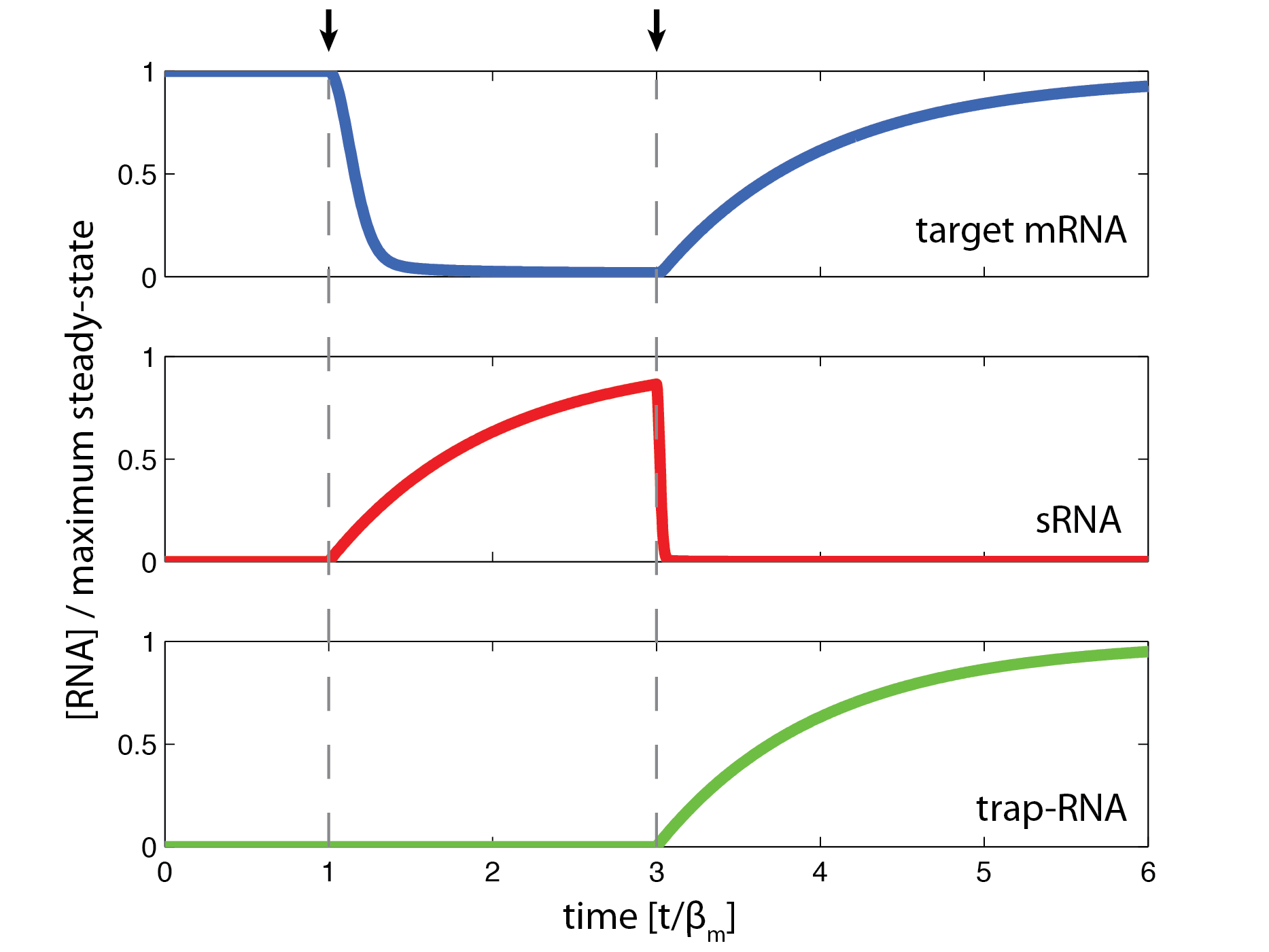
The temporal behavior is investigated using Runge-Kutta algorithm for numerical solution of differential equations. The equations used are the model 1 ODEs on a dimensionless form to facilitate the interpretation (see derivation). The parameters are based on estimates from literature. The simulation indicate a fast response time on the order of minutes when silencing target gene and a longer response time when reactivating the target gene.
The temporal behavior indicates the possibility of pulse experiments where any gene can be silenced or partly silenced upon induction and then subsequently reactivated.
Parameters and proposed experiments
In order to use the expressions for steady-state for empirical analysis the fold repression, $\phi$, must somehow be measurable. To arrive at some expression relating $\phi$ to empirical data, the steady-state of the expressed target gene is assumed to be proportional to the steady-state of the target mRNA. Using translational or transcriptional fusion of a reporter gene to the target gene the fold repression can be approximated by
\begin{equation} \phi \approx \frac{[A_{max}]}{[A]} \end{equation}
where $[A]$ is some measure proportional to the amount of reporter gene and $[A_{max}]$ is some measure at maximum expression. The measures of reporter gene could be either fluorescence from GFP or absorbance of X-gal product due to LacZ activity.
The parameters of $\lambda_s = \frac{\beta_m \beta_s}{k_s}$ and $\lambda_r = \frac{\beta_s \beta_r}{k_r}$, which arises in both steady-state solutions can be interpreted as leakage rates. In other words the ratio between the background degradation rate and the mediated specific degradation rate. The leakage rate $\lambda_s$ can be determined by fitting $\phi$ against $\alpha_s$. Similarly $\lambda_s$ and $\lambda_r$ can be determined by fitting $\phi$ to values of $\alpha_s$ and $\alpha_r$ using steady-state equations for either model 1 or model 2. The goodness of fit should provide evidence discerning the two alternative hypotheses of catalytic or partly stoichiometric trap-RNA.
The production terms $\alpha_m$, $\alpha_s$ and $\alpha_r$ can be constant or variable depending on inducers. Inducible promoter activity can be approximated by a simple linear function or by the Hill binding equation
\begin{equation} \alpha = \frac{\alpha_{max} [I]^n}{K_d + [I]^n} \end{equation}
where $[I]$ is the inducer concentration, $n$ is the Hill coefficient, $\alpha_{max}$ is the maximum production rate at full saturation and $K_d$ is the binding coefficient for the inducer-promoter complex.
The background degradation rates can be modeled as first order decay processes and determined by fitting to
\begin{equation} N(t) = N_0e^{-\beta t} \end{equation}
where $N(t)$ is the amount of RNA and intracellular production of RNA is stopped at $t=0$. Experiments indicate[3] that $\beta_s = \beta_m = 0.0257 min ^{-1}$.
Estimating the role of Hfq
Hfq is necessary for the system to work and inherently related to the kinetic $k_s$ and $k_r$ defined by
\begin{equation} k = \frac{k_1 k_2}{k_{-1} + k_2} \end{equation}
The dissociation constant is defined by $K_d = \frac{k_{-1}}{k_1}$. To relate $K_d$ to $k$ the on rate $k_1$ is assumed to be constant with respect to $K_d$ and any change in $K_d$ is assumed only to affect the off-rate $k_{-1}$. By inserting $k_{-1} = k_1 K_d$ it follows that
\begin{equation} \frac{1}{k} = \frac{1}{k_1} + \frac{1}{k_2} K_d \end{equation}
Using experimentally determined values of $k$ and $K_d$ prediction from secondary RNA structure predictors, eg. RNA fold or Vienna package, it is possible to investigate the relationship.
The role of Hfq in RNA-RNA hybridization has not been fully elucidated. A proposed mechanism is, that Hfq increases the on rate by some factor. If Hfq works by increasing the local concentration of RNA the factor would describe the increased probability of RNA collision caused by the presence of Hfq. Incorporating this idea we define the following altered on rate $k_{1} = \alpha_H k_{1}^{\circ}$ where $\alpha_H \geq 1$ and get \begin{equation} \frac{1}{k} = \frac{1}{\alpha_H k_1^{\circ}} + \frac{1}{k_2} K_d \end{equation} An expression which could guide experiments aimed at investigating the role of Hfq in post-transcriptional regulation.
Conclusion
The modeling of the trap-RNA system provides a framework for characterization and subsequent application in rational design or gene silencing experiments. The developed methods of characterization are general and applies to all potential target genes. The fold repression is independent on the amount of target mRNA, and hence system characterization is valid for any target mRNA expression level. This significantly simplifies applying the trap-RNA system because the trap-RNA system can be seen as an independent component simply lowering the expression by some factor. Temporal simulation of the model can be used to calculate the time necessary for steady-state to occur. The simulation indicates that gene silencing occurs fast, on the order of minutes, whereas reactivation is slower due to transcript build-up.
References
[1] Levine, Erel, Zhongge Zhang, Thomas Kuhlman, and Terence Hwa. Quantitative characteristics of gene regulation by small RNA. PLoS biology. 5, no. 9 (2007).
[2] Mitarai, Namiko, Julie-Anna M Benjamin, Sandeep Krishna, Szabolcs Semsey, Zsolt Csiszovszki, Eric Massé, and Kim Sneppen. Dynamic features of gene expression control by small regulatory RNAs. Proceedings of the National Academy of Sciences of the United States of America 106, no. 26 (2009): 10655-10659.
[3] Overgaard, Martin, Jesper Johansen, Jakob Møller‐Jensen, and Poul Valentin‐Hansen. Switching off small RNA regulation with trap‐mRNA. Molecular Microbiology 73, no. 5 (September 2009): 790-800. http://onlinelibrary.wiley.com/doi/10.1111/j.1365-2958.2009.06807.x/abstract.
 "
"


