Team:NTNU Trondheim/Modeling
From 2011.igem.org
(→Results) |
(→Results) |
||
| Line 103: | Line 103: | ||
[[File:variance.png|730x440px]] | [[File:variance.png|730x440px]] | ||
| - | Figure 5: '' | + | Figure 5: ''Variance and fano factor for increasing values of ppGpp'' |
== Model Validation == | == Model Validation == | ||
Revision as of 17:36, 20 September 2011

Modeling
To describe and understand the biological reactions and processes as the bacteria turns red under stress, we developed multiple mathematical and statistical models. As the most basic model we used a system of ordinary differential equations (ODE). This is a fully deterministic model, describing the change in concentration for all molecules involved.
Taking into account that the number of molecules in the cell, tends to be low and their movement random, one would have to use a model that allow randomness. This will result in a system of stochastic differential equations (SDE), which describe the underlying model from an observed pattern (random motion) in the number of molecules over time, given a concentration of ppGpp. A realization of such a model can be found under in figure in section for Results. Investigation of those models is done using Monte Carlo simulation in matlab and Dizzy.
Model introduction
At the heart of the modeling lies biological consistency and data integration. The modeling will be focused on interpretation simplicity and data consistency. That is to develop models that can be easily interpreted by biologist and mathematicians, but also describe what is observed at the laboratory.
The two main ways to model biological systems are deterministic and stochastic. In this project we will attempt to approach the problems in both ways. Using a deterministic model, with fixed parameters, and a stochastic model to integrate data more dynamically.
Process description
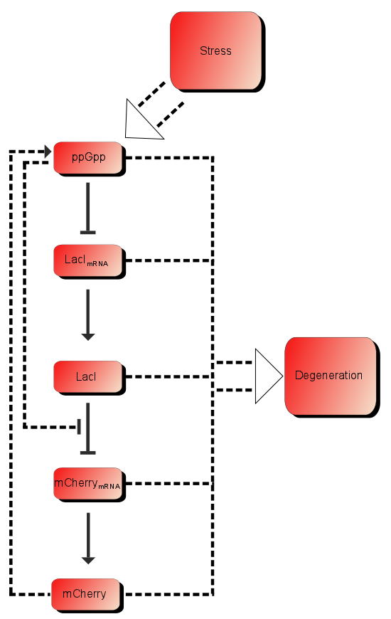
As described in the introduction, ppGpp will repress the production of LacI and LacI represses the production of mCherry. These are the dominating processes. In short, when ppGpp are not present there will be little mCherry and when ppGpp are present the level of mCherry will be substantially higher.
In addition to these processes there are additional processes which might be of importance. First of all ppGpp affects the RNAP (RNA polymerase) and can therefore affect the production of mCherry as well as the production of LacI. As described in the introduction LacI is expected to be heavily downregulated by ppGpp. The production of mCherry can also in some cases lead to stress and therefore more ppGpp which in turn leads to more mCherry, in other words a positive feedback loop. These effects are assumed to be small, but might still affect the outcome.
Figure 1:The processes involved in our system
The Models
Four basic models where constructed, which will be described below.
Systems of ODE
Models based on Ordinary Differential Equations (ODEs) are one of the most used methods of describing genetic circuits, while the different processes and reactions taking place in the cell are described by a set of coupled differential equations. This method might give both qualitative and quantitative information about the system and can therefore be very useful. It is however dependent on accurate kinetic reaction parameters and in some cases one also has to take into account the stochastic nature of genetic circuits. The equations are then solved either in Dizzy or Matlab.
Basic Model
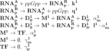
Based on the model above the most important processes are, the symbols to the left of the equation denotes the kinetic parameter for the process:
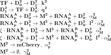
The first process describes ppGpp attaching to the RNA polymerase, RNApA denotes the active part which is not repressed by ppGpp. RNApR is the number of repressed RNA polymerase molecules. This process can also be reversed. The transcription of mRNA is described in one step. D01 is the promoter determining the production of LacI mRNA and M1 is LacI mRNA. The LacI mRNA in turn leads to production of LacI transcription factor denoted as TF. Both mRNA and LacI is degraded as well. LacI will then inhibit mCherry:
Where D12 denotes promotors inhibited by LacI transcription factor. ξ is a measure of how strongly ppGpp affects mCherry directly, if 1 it is unaffected if 0 it is affected as strongly as LacI.
Steady State
Since it is difficult to find accurate parameters for all the processes involved and since it is often only the concentrations in steady state (long after the stress was first induced) that can be measured, all quantities involved were assumed to be constant. This assumption simplifies the system greatly and reduced the problem to these two equations:
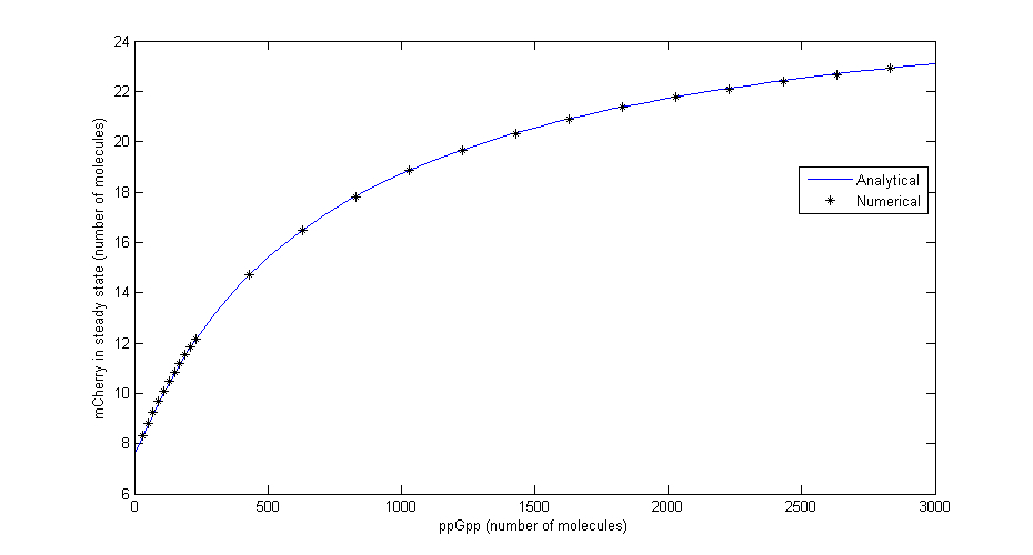
Where Ci=αMiαpiRNApT/γMiγpi, RNApT is the total number of RNA-polymerase molecules in the cell and Ki=qi/ki. To check that the equations for steady state are correct a comparison was made between the numerical solution in Dizzy and the analytical solution for different levels of ppGpp. The comparison shown in the figure below shows that there is excellent agreement.
Figure 2: Comparison between numerical simulation and analytical solution in steady state for different values of ppGpp
Stochastic Differential equations
In the cell, all movement of the molecules is random, this gives rise to the stochasticity observed in gene expression experiment. In this section we outline two methods where the randomness is accounted for; the Gillespie algorithm and the approximation τ - leap algorithm.
When the number of participating molecules are low (which do happen in the cell), then stochasticity really matters. If there are many molecules, then the behavior of the reactions goes "smooth" and looks like an ODE. However when to number of reactants gets small, the number of reactions in a small time frame varies, this gives rise to the irregularity seen in the time series for the number of created products in the cell.
Gillespie
The Gillespie algorithm is a model that simulates the number of reactions and the time between the reactions exactly (under some assumptions). The most important assumptions is that the concentration of the reactants is distributed uniformly in the cell, the other important assumption is that the time between the reactions occur is markovian, that is it has no memory of how long the previous time step was.
An improved version of the original algorithm, the Gibson-Bruck algorithm, was used with Dizzy.
Tau - leap Algorithm
Instead of calculating the time between each reaction, we can fix a time frame and estimate how many reactions occur in that time frame.
It can be shown that setting the production and destruction rate from the ODE in as a rate parameter in an Poisson distribution, will give the same result. This is a nice way of reconfiguring the tau - leap such that it gives a clear and precise relation to the ODE models, and mathematical consistency.
This approach was used to create a framework for a stochastic simulation using the computer language C++, there where an attempt to make this in a fully functional open source program. However this attempt stranded due to lack of time.
Results
This section describes the findings from the theoretical model presented in the equations above.
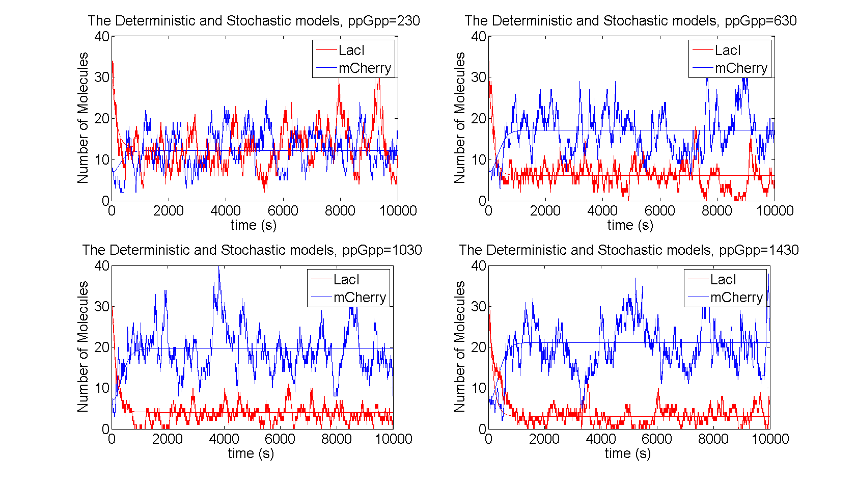
As seen in figure 3 the level of LacI is reduced when ppGpp increases in the cell, which in turn leads to increased level of mCherry. The level of LacI reaches a saturation point, since there will be some production of LacI due to leakage, this sets a limit from above for mCherry. The stochastic realization fluctuates around the deterministic results, with the distributions shown in figure 4.
Figure 3:The number of molecules of the proteins for the stochastic and the deterministic models are shown for different values of ppGpp
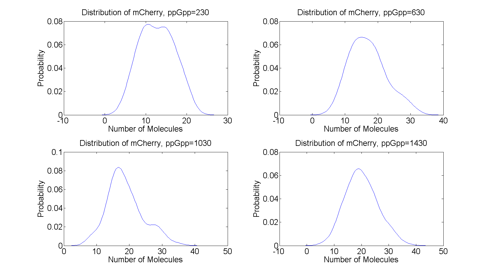
All the distributions are unimodal having only one peak, peaked around the steady state value from the deterministic model. The distributions for ppGpp=630 and ppGpp=1030 have heavy tails which indicates larger deviations from the mean value, while the distributions for ppGpp=230 and ppGpp=1430 are more symmetric, resembling the normal distribution.
Figure 4:The distribution of mCherry for t=2000s to t=10000s for different values of ppGpp
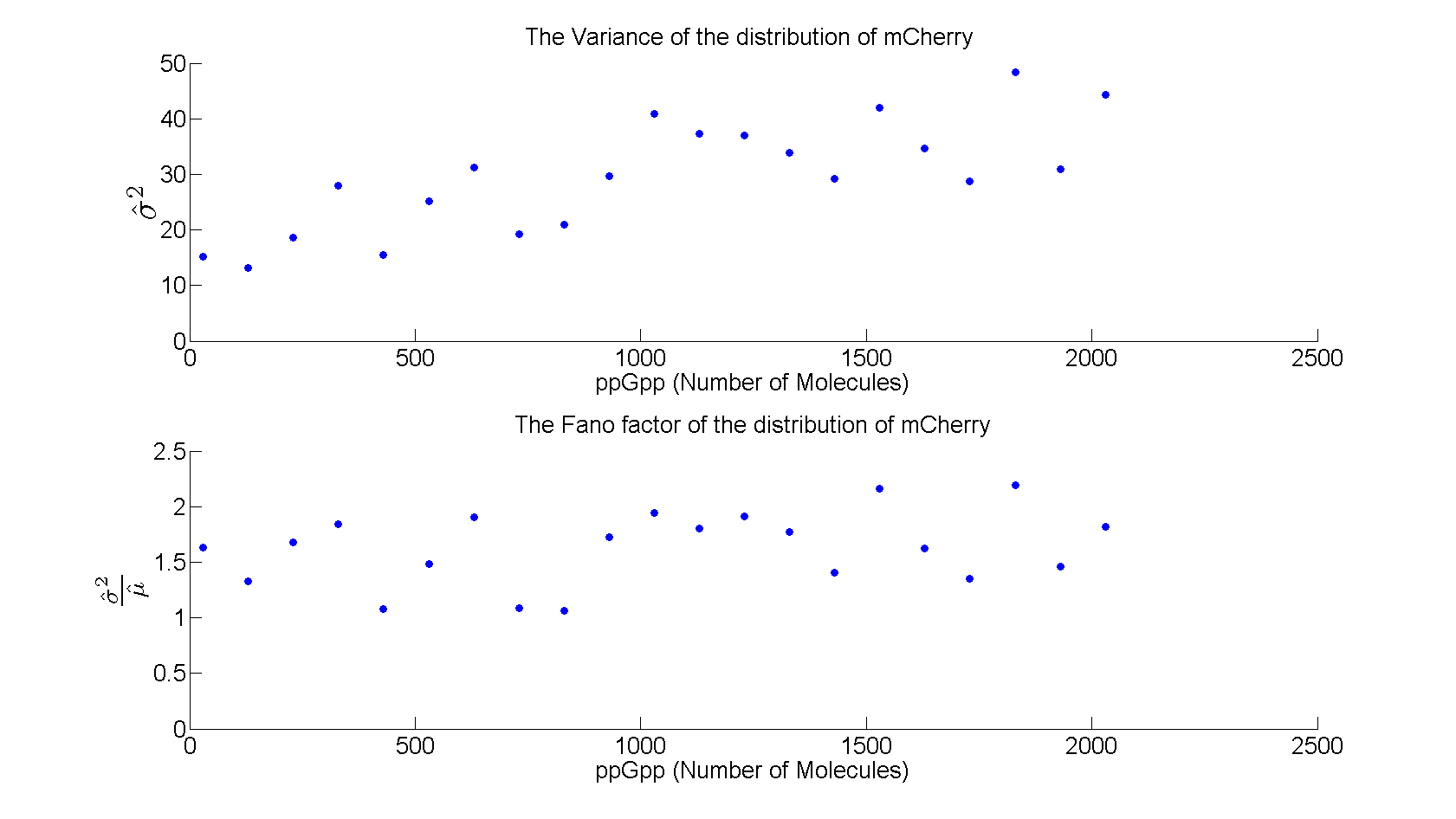
As shown in figure the variance increases linearly with increasing level of ppGpp, while the fanofactor (σ2/μ) is almost constant around 1.5 .
Figure 5: Variance and fano factor for increasing values of ppGpp
Model Validation
To see if the results agree with the theoretical model is vital in all parts of science. In this section we will give a short reasoning of why our models seems to fit the observed data. Here we will consider our model in two distinct parts, one deterministic model and one stochastic model, both of equally importance.
Because of the limited amount of data currently available it is diffucult to draw conclusions. In the modeling the level of ppGpp was assumed known, however we do not know at present the relationship between a stress level and the number of ppGpp and the relationship between the number of mCherry molecules and the flourescence level is also unknown.
 "
"


