Team:Wageningen UR/Project/ModelingProj1
From 2011.igem.org
(→Modeling synchronized oscillations) |
(→Modeling synchronized oscillations) |
||
| Line 28: | Line 28: | ||
{{:Team:Wageningen_UR/Templates/Style | text= __NOTOC__ | {{:Team:Wageningen_UR/Templates/Style | text= __NOTOC__ | ||
| - | === | + | === Short repetition of the Hasty construct used as base for our system === |
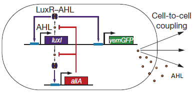
For a better understanding of the equations which were used for the modeling of the system, figure 1 shows a short repetition of the circuit published by Danino et al. in the paper [http://www.nature.com/nature/journal/v463/n7279/abs/nature08753.html “A synchronized quorum of genetic clocks”], in our team commonly referred to as the "Hasty construct", which was used as a base for our design. | For a better understanding of the equations which were used for the modeling of the system, figure 1 shows a short repetition of the circuit published by Danino et al. in the paper [http://www.nature.com/nature/journal/v463/n7279/abs/nature08753.html “A synchronized quorum of genetic clocks”], in our team commonly referred to as the "Hasty construct", which was used as a base for our design. | ||
| Line 44: | Line 44: | ||
| - | === | + | === Mathematical model of the Hasty construct === |
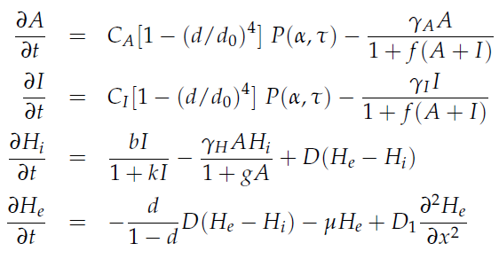
| - | Since our bio bricked oscillatory system is based on the design seen above, our first model of the system is a reproduction of the mathematical model in the [http://www.nature.com/nature/journal/v463/n7279/suppinfo/nature08753.html supplementary information] accompanying the publication mentioned. In their simulations, Danino et al. used the following set of delay differential equations, which we also used for our modeling | + | Since our bio bricked oscillatory system is based on the design seen above, our first model of the system is a reproduction of the mathematical model in the [http://www.nature.com/nature/journal/v463/n7279/suppinfo/nature08753.html supplementary information] accompanying the publication mentioned. In their simulations, Danino et al. used the following set of delay differential equations, which we also used as starting point for our modeling work. }} |
[[File:Equations_hasty_WUR.png|350px|left]] | [[File:Equations_hasty_WUR.png|350px|left]] | ||
| Line 77: | Line 77: | ||
in which tau represents the time step. It can be seen that the function takes the history of the system into account, since the production of the proteins depend on the past concentration of internal AHL as in: [[File:Equations3_hasty_WUR.png]]. | in which tau represents the time step. It can be seen that the function takes the history of the system into account, since the production of the proteins depend on the past concentration of internal AHL as in: [[File:Equations3_hasty_WUR.png]]. | ||
| - | |||
| - | |||
| - | |||
| + | === Writing a modeling tool in matlab === | ||
[[File:Oscillation_GUI_WUR.png|center]] | [[File:Oscillation_GUI_WUR.png|center]] | ||
| Line 86: | Line 84: | ||
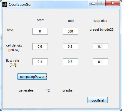
'''Fig.2:''' ''GUI of the matlab modeling tool created by team Wageningen UR'' | '''Fig.2:''' ''GUI of the matlab modeling tool created by team Wageningen UR'' | ||
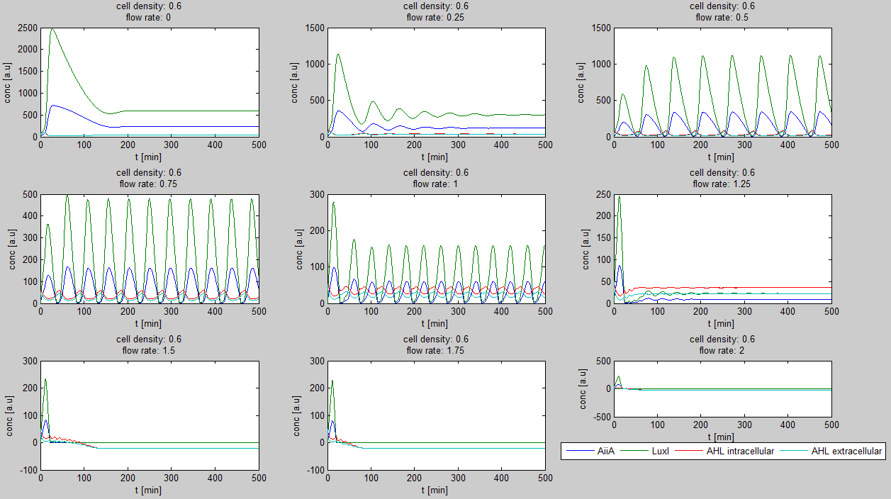
| - | - | + | For the first simulations, the same values for the parameters were used as in the cited paper and can be found in the [http://www.nature.com/nature/journal/v463/n7279/suppinfo/nature08753.html supplementary information]. To get graphs representing optimal oscillations, our team created a script for a matlab modeling tool which uses nested for-loops to vary the flow rate and cell density over a range of values. The resulting tool allows the user to enter the range in which the variables should be varied. The tool then iterates over the values and plots graphs of all combinations possible for that range of values. Figure 2 shows an example output of the tool. |
| + | |||
[[File:Example_output_graphs_WUR.png|700px|center]] | [[File:Example_output_graphs_WUR.png|700px|center]] | ||
| Line 97: | Line 96: | ||
| - | === | + | === Conclusions for our system === |
The first observation from the model was that, for oscillations to occur, the flow rates may not be too fast, especially at lower cell densities. Since the device used for our system has larger dimensions than the microfluidic device used by Danino et al. the flow rates in the velocities required could not be achieved by varying height differences alone. Further information can be found in the information about the [[Team:Wageningen_UR/Project/Devices#2._Setup| platform used to measure oscillations.]] | The first observation from the model was that, for oscillations to occur, the flow rates may not be too fast, especially at lower cell densities. Since the device used for our system has larger dimensions than the microfluidic device used by Danino et al. the flow rates in the velocities required could not be achieved by varying height differences alone. Further information can be found in the information about the [[Team:Wageningen_UR/Project/Devices#2._Setup| platform used to measure oscillations.]] | ||
| Line 106: | Line 105: | ||
| - | === | + | === Expansion of the model for the double tunable oscillatory construct === |
To accomodate the idea of the [[Team:Wageningen_UR/Project/CompleteProject1Description| double tunable oscillator]], the original set of delay differential equations shown above was expanded by two additional differential equations showing the behaviour of the lacI and tetR repressor. The equations for the LuxI and AiiA production were then expanded by a term showing the influence of the corresponding repressor lacI for LuxI and tetR for Aiia respectively. Figure 3. shows the adjusted set of differential equations. | To accomodate the idea of the [[Team:Wageningen_UR/Project/CompleteProject1Description| double tunable oscillator]], the original set of delay differential equations shown above was expanded by two additional differential equations showing the behaviour of the lacI and tetR repressor. The equations for the LuxI and AiiA production were then expanded by a term showing the influence of the corresponding repressor lacI for LuxI and tetR for Aiia respectively. Figure 3. shows the adjusted set of differential equations. | ||
Revision as of 22:33, 18 September 2011
 "
"


