Team:NTNU Trondheim/Modeling
From 2011.igem.org
m |
(→Basic Model) |
||
| Line 40: | Line 40: | ||
Where '''D<sub>1</sub><sup>2</sup>''' denotes promotors inhibited by LacI transcription factor. It is assumed that ppGpp will not inhibit mCherry as strong as LacI. | Where '''D<sub>1</sub><sup>2</sup>''' denotes promotors inhibited by LacI transcription factor. It is assumed that ppGpp will not inhibit mCherry as strong as LacI. | ||
| + | ====Steady State==== | ||
| + | Since it is difficult to find accurate parameters for all the processes involved and since it is often only the concentrations in steady state (long after the stress was first induced) that can be measured the equations was solved for equilibrium. The following two equations was obtained: | ||
=== Stochastic Differential equations === | === Stochastic Differential equations === | ||
Revision as of 11:01, 4 September 2011

Modeling
To describe and understand the biological reactions and process, as the bacteria turns red under stress we developed multiple mathematical and statistical models. As the most basic model we used a system om ordinary differential equations (ODE), this is a fully deterministic model, describing the change in concentration for all molecules involved. The process for a bacteria to go from normal to glowing red is involved, and one can think of this as a stochastic process, that at each step, the process can ether succeed or fail, with a given probability. This gives rise to a Bayesian model.
Combining these two models will result in a system of stochastic differential equations (SDE), which will be solved using numerical algorithms. As a last model we will explore the relationship between variants of stress and fluoricene intensity using (non)-conventional regression.
Model Introduction
At the heart of the modeling lies biological consistency and data integration. The modeling will be focused on interpretation simplicity and data consistency. That is to develop models that can be easily interpreted by biologist and mathematicians, but the models should also strive to describe that which is observed at the laboratory.
The two main ways to model biological systems. One way is deterministic, the other is stochastic. In this project we will attempt to approach to problems in both ways. Using a deterministic model, with fixed parameters, and a stochastic model to integrate data more dynamically.
Process description
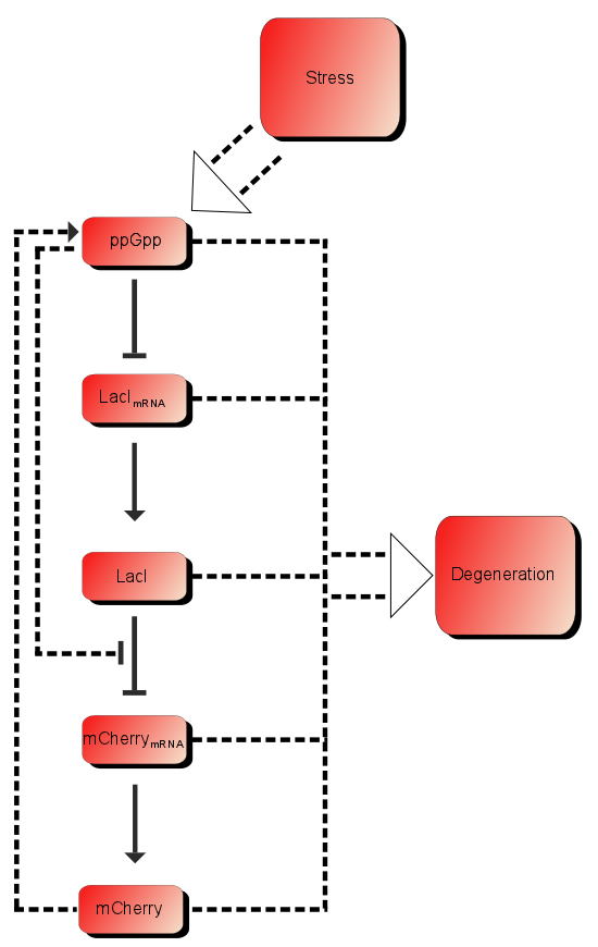
As described in the introduction, ppGpp will repress the production of LacI mRNA which in turn will increase the production of LacI. LacI will in turn repress the production of mCherry mRNA which leads to more mCherry. These are the dominating processes. In short when ppGpp are not present there will be little mCherry, when there are ppGpp rhe level of mCherry will be substantially higher.
In addition to these processes there are additional processes which might be of importance. First of all ppGpp affects the RNAp and can therefore affect the production of mCherry as well as the production of LacI, as described in the introduction LacI is expected to be heavily downregulated by ppGpp. The production of mCherry can also in some cases lead to stress and therefore more ppGpp which in turn leads to more mCherry, in other words a positive feedback loop. These effects are assumed to be small, but might still affect the outcome.
The Models
Four basic models where constructed, which will be described below.
File:ModelAssuptions.pdf File:ModelOvervew.pdf
Systems of ODE
Models based on Ordinary Differential Equations (ODEs) are one of the most used methods of describing genetic cicuits, the different processes and reactions taking place in the cell are described by a set of coupled differential equations. This method might give both qualitative and quantitative information about the system and can therefore be very useful. It is however dependent on accurate kinetic reaction parameters and in some cases one also has to take into account the stochastic nature of genetic circuits. The equations are then solved either in Dizzy or Matlab.
Basic Model
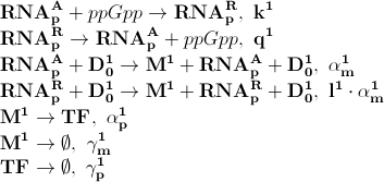
Based on the model above the most important processes are:
The first process describes ppGpp attaching to the RNA polymerase, RNApA denotes the active part which is not repressed by ppGpp. RNApR is the number of repressed RNA polymerase molecules. This process can also be reversed. The transcription of mRNA is described in one step. D01 is the promoter determining the production of LacI mRNA and M1 is LacI mRNA. The LacI mRNA in turn leads to production of LacI transcription factor denoted as TF. Both mRNA and LacI is degraded as well. LacI will then inhibit mCherry:
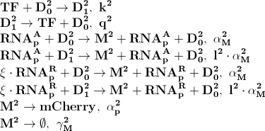
Where D12 denotes promotors inhibited by LacI transcription factor. It is assumed that ppGpp will not inhibit mCherry as strong as LacI.
Steady State
Since it is difficult to find accurate parameters for all the processes involved and since it is often only the concentrations in steady state (long after the stress was first induced) that can be measured the equations was solved for equilibrium. The following two equations was obtained:
Stochastic Differential equations
In the cell, all movement of the molecules is random, this gives rise to the stochasticity observed in gene expression experiment. In this section we outline two methods where the randomness is accuared for; the Gillespie algorithm and the approximation τ - leap algorithm.
When the number of participating molecules are low (which do happen in the cell), then stochasticity really matters. If there are many molecules, then the behavior of the reactions goes "smooth" and looks like an ODE. However when to number of reactants gets small, the number of reactions in a small time frame varies, this gives rise to the irregularity seen in the time series for the number of created products in the cell.
Gillespie
The Gillespie algorithm is a model that simulates the number of reactions and the time between the reactions exactly (under some assumptions). The most important assumptions is that the concentration of the reactants is distributed uniformly in the cell, the other important assumption is that the time between the reactions occur is markovian, that is it has no memory of how long the previous time step was.
Simulated and investigated using the program tool Dizzi, for system biology.
Tau - leap Algorithm
Instead of calculating the time between each reaction, we can fix a time frame and estimate how many reactions occur in that time frame.
It can be shown that setting the production and destruction rate from the ODE in as a rate parameter in an Poisson distribution, will give the same result. This is a nice way of reconfiguring the tau - leap such that it gives a clear and precise relation to the ODE models, and mathematical consistency.
This approach was used to write our one computer program for simulating any process in the cell using the tau - leap algorithm (see result for further information (coming soon) ).
Regression Models
As the level of stress grow, so will the number of mCherry molecules to, but how exactly are the relationship there? Using a flocytometry, we can measure the fluorescence in each cell, this will correspond to the amount of mCherry in the cell. For each stress level inn the experiment there will be a sample point for the concentration of mCherry with unequal variance (heteroscedasticity), this poses a major concern in the model as it brakes one of the fundamental assumptions in conventional regression. Whoever, using non - linear regression, this problem can be avoided with an unequal wight on each point in the regression curve.
To assess the relationship between levels of stress and production of mCherry (assuming steady state) we will use a smoothing spline with wights equal to the inverse of the variance at each point.
Model Validation
No data yet.
Bayesian Hierarchy
This model did not work properly, and was dropped to concentrate our effort on the other models.
As shown in the introduction, the process before the bacteria turns red is a linear chain of events. This can be modeled as a stochastic process, and solved with Monte Carlo methods. This is a way of including stochastic elements and data integration. Setting the probability of a transition to be successful within a time dt to be Beta distributed, with hyper parameters ("known constants"), αi and βi, the the probability of total success, that the start input will transcend and cause the output (observable), is the product of all the beta distributed variables, which itself is Beta distributed whit parameter α = ∑ αi-q+1 and β = ∑ βi-q+1, where q is the number of parameters.
Having done some previous test at the lab, we wish to extend this in a probabilistic context. To integrate this data and the model assumptions, we can get a better picture of what is happening in the cell, and how likely it is to succeed in each trail.
References
 "
"


